 EXAMINATIONS – 2022
Test One
EEEN 320
Signals, Systems and Statistics 2
Time Allowed:
EXAMINATIONS – 2022
Test One
EEEN 320
Signals, Systems and Statistics 2
Time Allowed:
50 minutes
CLOSED BOOK
Permitted materials: Only silent non-programmable calculators or silent programmable calcula-
tors with their memories cleared are permitted in this examination. A double
sided sheet of A4 paper with notes is also permitted (to be submitted).
Instructions:
Attempt ALL Questions
The test will be marked out of a total of 50 marks.
Name: .......................................
EEEN 320
Page
1 of
17
Student ID: . . . . . . . . . . . . . . . . . . . . . . .
1.
Confidence Interval 1
(7 marks)
A 99% confidence interval for a population mean based on a sample size of 64 is computed
to be (16.3, 18.7). How large a sample is needed so that a 99% confidence interval will
specify the mean to be within ±1.0%?
EEEN 320
Page
2 of
17
Student ID: . . . . . . . . . . . . . . . . . . . . . . .
2.
Confidence Interval 2
(20 marks)
The temperature of a certain solution is estimated by taking a large number of independent
measurements and averaging them. The estimate is 37o C, and the uncertainty (standard
deviation) in this estimate is 0.1oC.
(a) Find a 95% confidence interval for the temperature
(7 marks)
(b) What is the confidence level of the interval 37 ± 0.1o C?
(5 marks)
(c) If only a small number of independent measurements had been made, what additional
assumption would be necessary in order to compute a confidence interval?
(3 marks)
(d) Making the additional assumption, compute a 95% confidence interval for the tem-
perature if 10 measurements were made.
(5 marks)
EEEN 320
Page
3 of
17
Student ID: . . . . . . . . . . . . . . . . . . . . . . .
3.
Hypothesis Testing 1
(8 marks)
In a sample of 150 households in a certain city, 110 had high-speed internet access. Can
you conclude that more than 70% of the households in this city have high-speed internet
access?
EEEN 320
Page
4 of
17
Student ID: . . . . . . . . . . . . . . . . . . . . . . .
4.
Hypothesis Testing 2
(15 marks)
(a) A new post-surgical treatment is being compared with a standard treatment. Seven
subjects receive the new treatment, while seven others (the controls) receive the stan-
dard treatment. The recovery times, in days, are as follows
Treatment X
12
13
15
19
20
21
27
Control Y
18
23
24
30
32
35
40
There is no evidence that the recovery times follow a Gaussian distribution. Can you
conclude that the mean rate differs between the treatment and control?
(10 marks)
(b) Describe a second approach to finding the p-value for the above hypothesis if more
subjects (both for the treatment group and the control group) were available.
(5 marks)
EEEN 320
Page
5 of
17
Tables for ECEN321
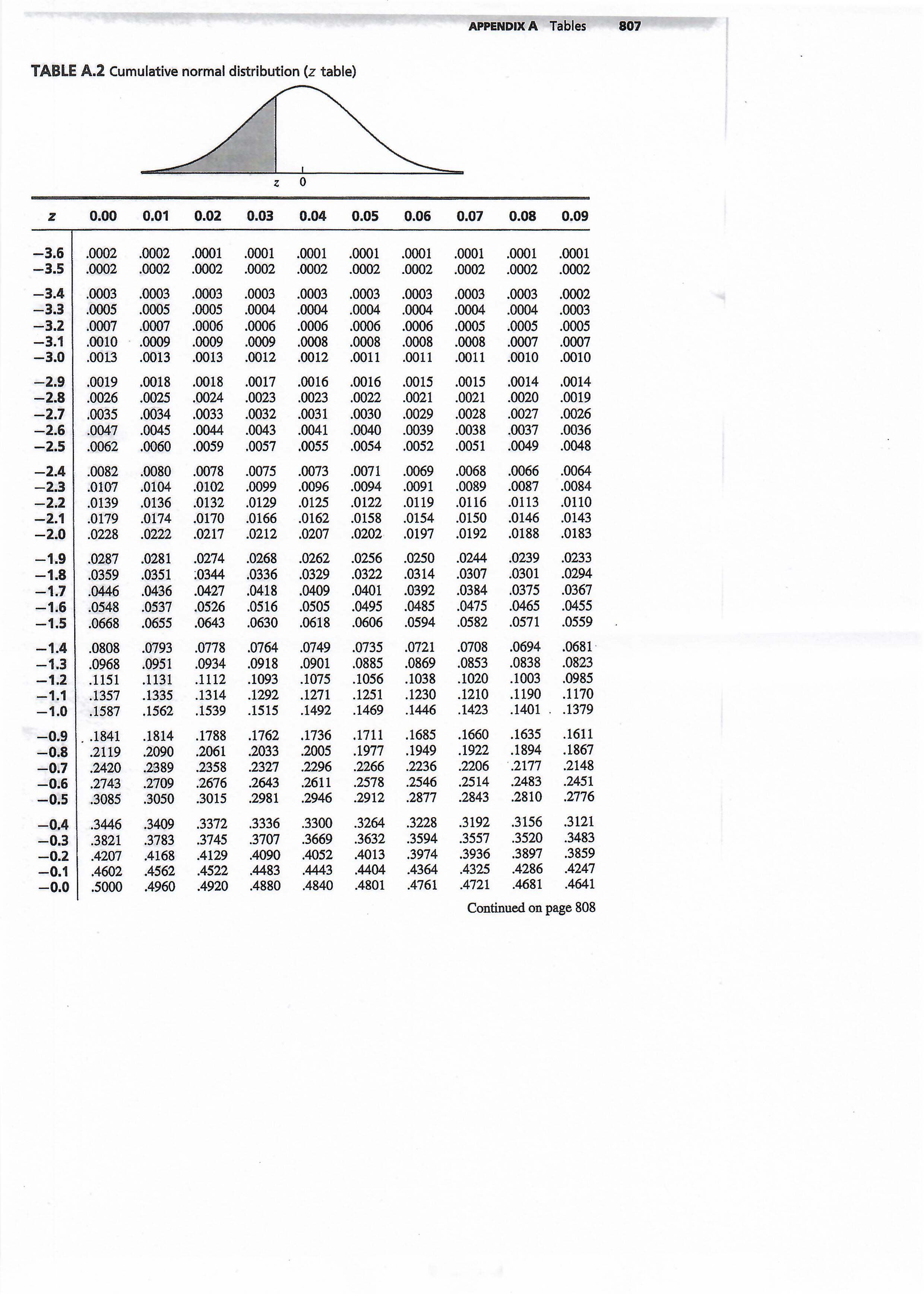
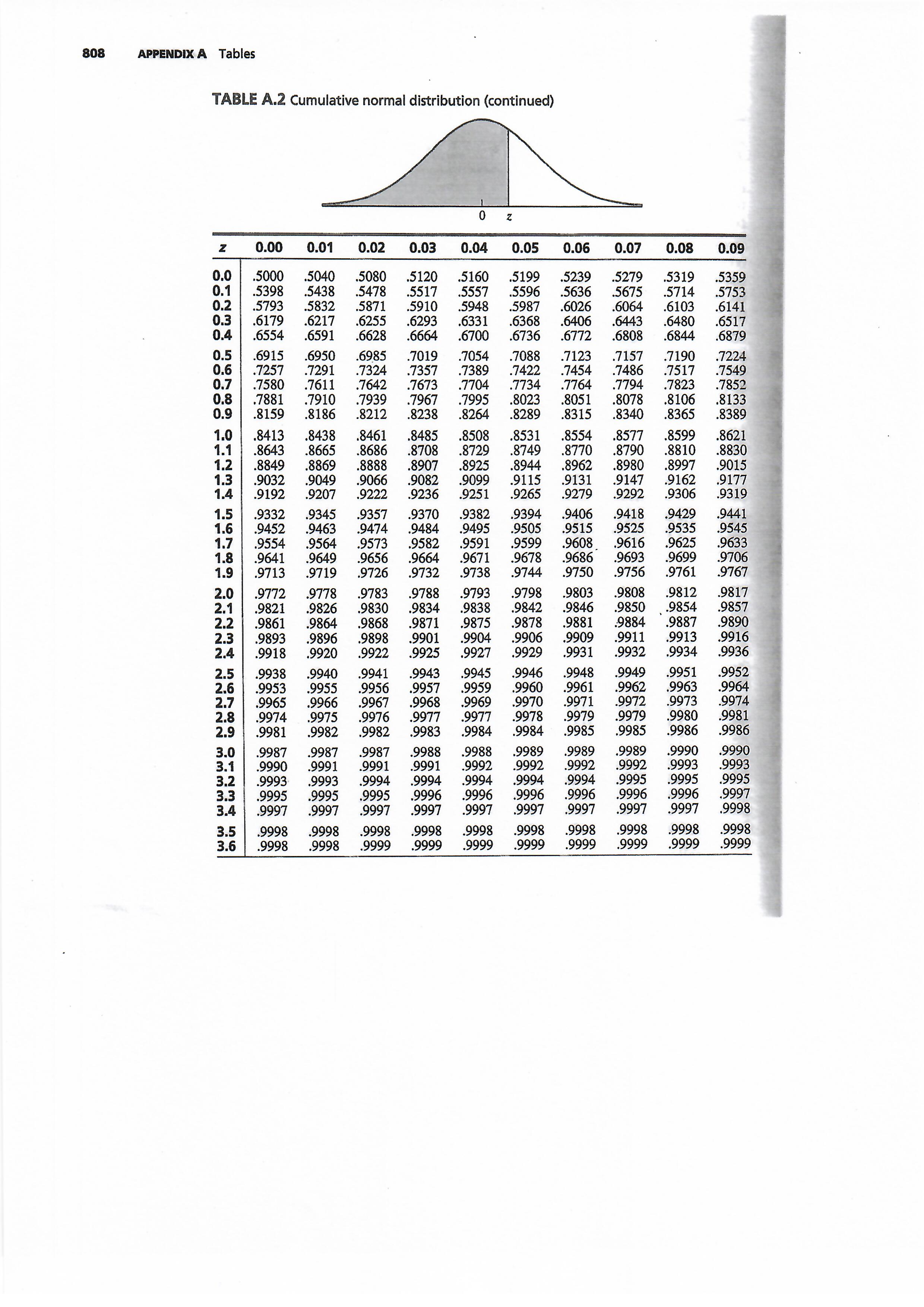
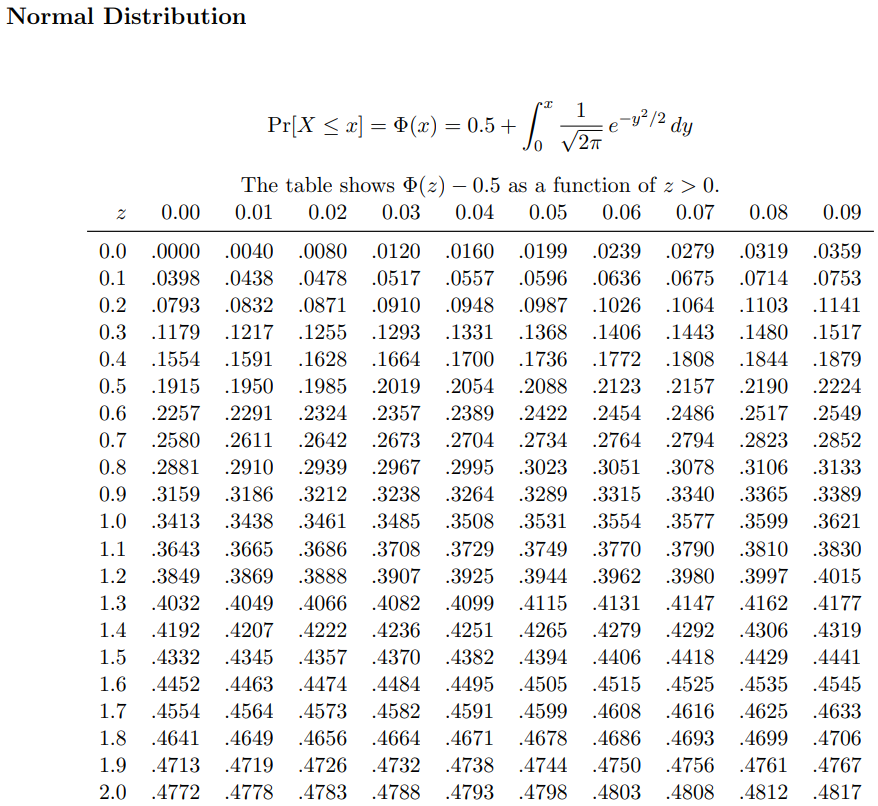
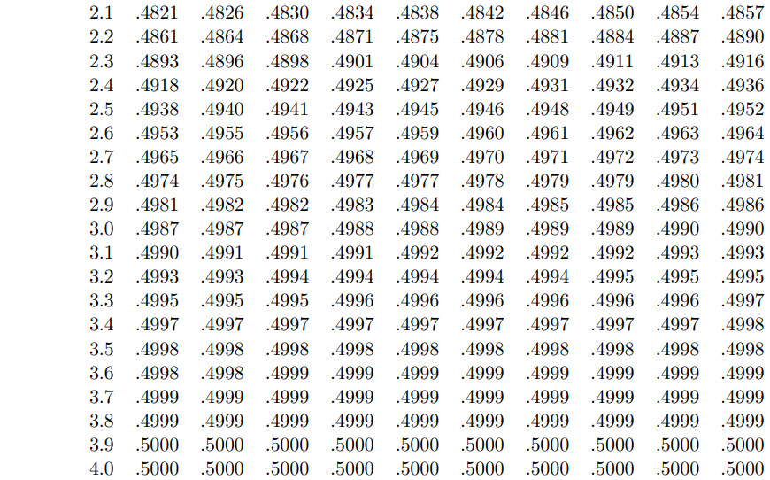
Normal Distribution
Z x 1
Pr[X ≤ x] = Φ(x) = 0.5 +
√
e−y2/2 dy
0
2π
The table shows Φ(z) − 0.5 as a function of z > 0.
z
0.00
0.01
0.02
0.03
0.04
0.05
0.06
0.07
0.08
0.09
0.0
.0000
.0040
.0080
.0120
.0160
.0199
.0239
.0279
.0319
.0359
0.1
.0398
.0438
.0478
.0517
.0557
.0596
.0636
.0675
.0714
.0753
0.2
.0793
.0832
.0871
.0910
.0948
.0987
.1026
.1064
.1103
.1141
0.3
.1179
.1217
.1255
.1293
.1331
.1368
.1406
.1443
.1480
.1517
0.4
.1554
.1591
.1628
.1664
.1700
.1736
.1772
.1808
.1844
.1879
0.5
.1915
.1950
.1985
.2019
.2054
.2088
.2123
.2157
.2190
.2224
0.6
.2257
.2291
.2324
.2357
.2389
.2422
.2454
.2486
.2517
.2549
0.7
.2580
.2611
.2642
.2673
.2704
.2734
.2764
.2794
.2823
.2852
0.8
.2881
.2910
.2939
.2967
.2995
.3023
.3051
.3078
.3106
.3133
0.9
.3159
.3186
.3212
.3238
.3264
.3289
.3315
.3340
.3365
.3389
1.0
.3413
.3438
.3461
.3485
.3508
.3531
.3554
.3577
.3599
.3621
1.1
.3643
.3665
.3686
.3708
.3729
.3749
.3770
.3790
.3810
.3830
1.2
.3849
.3869
.3888
.3907
.3925
.3944
.3962
.3980
.3997
.4015
1.3
.4032
.4049
.4066
.4082
.4099
.4115
.4131
.4147
.4162
.4177
1.4
.4192
.4207
.4222
.4236
.4251
.4265
.4279
.4292
.4306
.4319
1.5
.4332
.4345
.4357
.4370
.4382
.4394
.4406
.4418
.4429
.4441
1.6
.4452
.4463
.4474
.4484
.4495
.4505
.4515
.4525
.4535
.4545
1.7
.4554
.4564
.4573
.4582
.4591
.4599
.4608
.4616
.4625
.4633
1.8
.4641
.4649
.4656
.4664
.4671
.4678
.4686
.4693
.4699
.4706
1.9
.4713
.4719
.4726
.4732
.4738
.4744
.4750
.4756
.4761
.4767
2.0
.4772
.4778
.4783
.4788
.4793
.4798
.4803
.4808
.4812
.4817
2.1
.4821
.4826
.4830
.4834
.4838
.4842
.4846
.4850
.4854
.4857
2.2
.4861
.4864
.4868
.4871
.4875
.4878
.4881
.4884
.4887
.4890
2.3
.4893
.4896
.4898
.4901
.4904
.4906
.4909
.4911
.4913
.4916
2.4
.4918
.4920
.4922
.4925
.4927
.4929
.4931
.4932
.4934
.4936
2.5
.4938
.4940
.4941
.4943
.4945
.4946
.4948
.4949
.4951
.4952
2.6
.4953
.4955
.4956
.4957
.4959
.4960
.4961
.4962
.4963
.4964
2.7
.4965
.4966
.4967
.4968
.4969
.4970
.4971
.4972
.4973
.4974
2.8
.4974
.4975
.4976
.4977
.4977
.4978
.4979
.4979
.4980
.4981
2.9
.4981
.4982
.4982
.4983
.4984
.4984
.4985
.4985
.4986
.4986
3.0
.4987
.4987
.4987
.4988
.4988
.4989
.4989
.4989
.4990
.4990
3.1
.4990
.4991
.4991
.4991
.4992
.4992
.4992
.4992
.4993
.4993
3.2
.4993
.4993
.4994
.4994
.4994
.4994
.4994
.4995
.4995
.4995
3.3
.4995
.4995
.4995
.4996
.4996
.4996
.4996
.4996
.4996
.4997
3.4
.4997
.4997
.4997
.4997
.4997
.4997
.4997
.4997
.4997
.4998
3.5
.4998
.4998
.4998
.4998
.4998
.4998
.4998
.4998
.4998
.4998
3.6
.4998
.4998
.4999
.4999
.4999
.4999
.4999
.4999
.4999
.4999
3.7
.4999
.4999
.4999
.4999
.4999
.4999
.4999
.4999
.4999
.4999
3.8
.4999
.4999
.4999
.4999
.4999
.4999
.4999
.4999
.4999
.4999
3.9
.5000
.5000
.5000
.5000
.5000
.5000
.5000
.5000
.5000
.5000
4.0
.5000
.5000
.5000
.5000
.5000
.5000
.5000
.5000
.5000
.5000
1
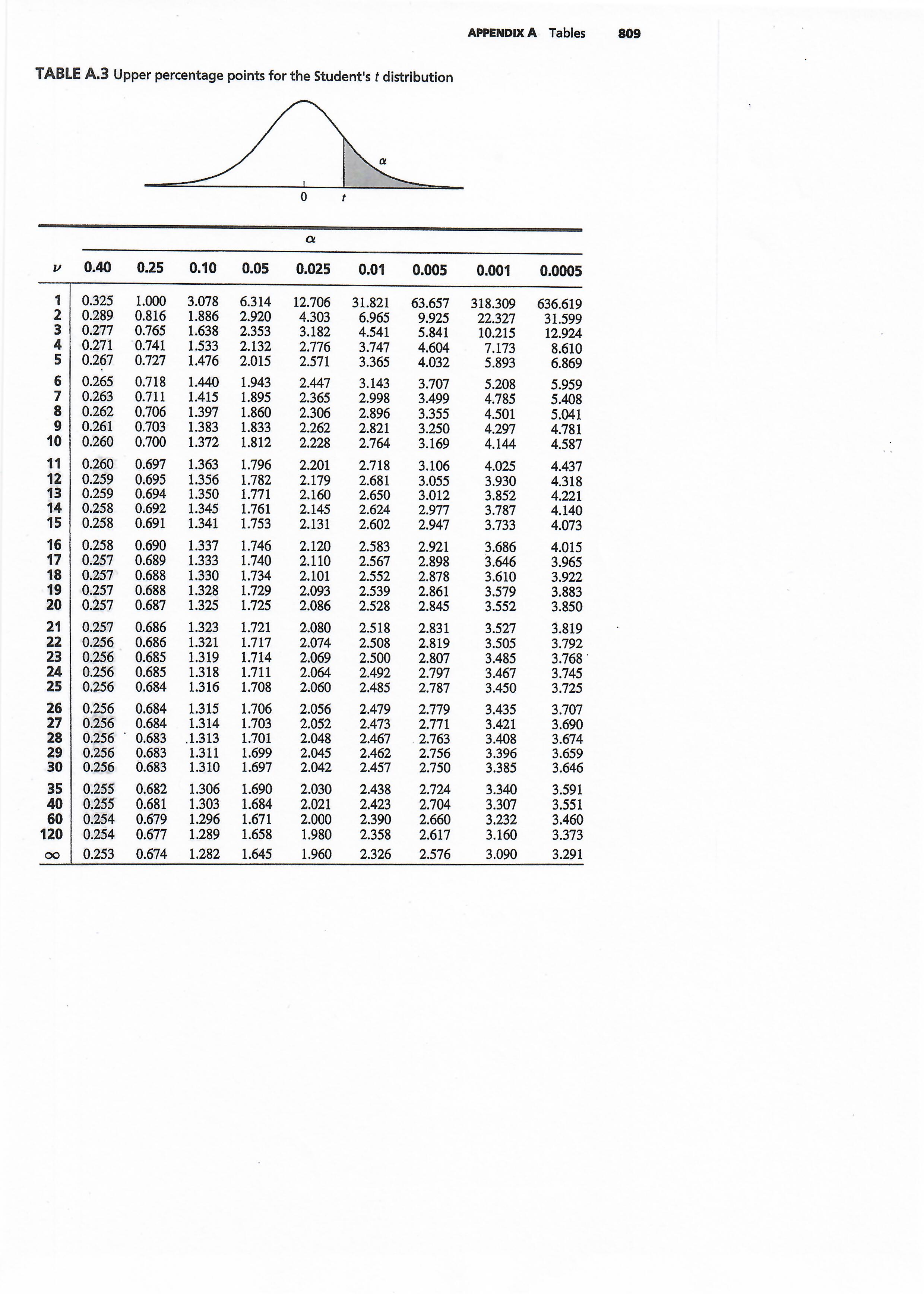
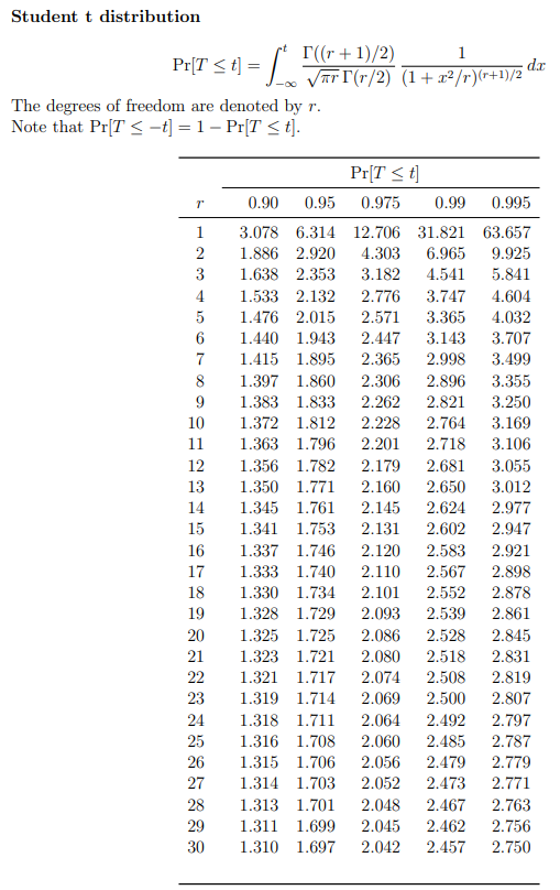
Student t distribution
Z t Γ((r + 1)/2)
1
Pr[T ≤ t] =
√
dx
−∞
πr Γ(r/2) (1 + x2/r)(r+1)/2
The degrees of freedom are denoted by r.
Note that Pr[T ≤ −t] = 1 − Pr[T ≤ t].
Pr[T ≤ t]
r
0.90
0.95
0.975
0.99
0.995
1
3.078 6.314 12.706 31.821 63.657
2
1.886 2.920
4.303
6.965
9.925
3
1.638 2.353
3.182
4.541
5.841
4
1.533 2.132
2.776
3.747
4.604
5
1.476 2.015
2.571
3.365
4.032
6
1.440 1.943
2.447
3.143
3.707
7
1.415 1.895
2.365
2.998
3.499
8
1.397 1.860
2.306
2.896
3.355
9
1.383 1.833
2.262
2.821
3.250
10
1.372 1.812
2.228
2.764
3.169
11
1.363 1.796
2.201
2.718
3.106
12
1.356 1.782
2.179
2.681
3.055
13
1.350 1.771
2.160
2.650
3.012
14
1.345 1.761
2.145
2.624
2.977
15
1.341 1.753
2.131
2.602
2.947
16
1.337 1.746
2.120
2.583
2.921
17
1.333 1.740
2.110
2.567
2.898
18
1.330 1.734
2.101
2.552
2.878
19
1.328 1.729
2.093
2.539
2.861
20
1.325 1.725
2.086
2.528
2.845
21
1.323 1.721
2.080
2.518
2.831
22
1.321 1.717
2.074
2.508
2.819
23
1.319 1.714
2.069
2.500
2.807
24
1.318 1.711
2.064
2.492
2.797
25
1.316 1.708
2.060
2.485
2.787
26
1.315 1.706
2.056
2.479
2.779
27
1.314 1.703
2.052
2.473
2.771
28
1.313 1.701
2.048
2.467
2.763
29
1.311 1.699
2.045
2.462
2.756
30
1.310 1.697
2.042
2.457
2.750
2
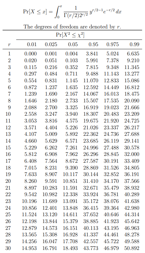
Chi-square distribution
Z x
1
Pr[X ≤ x] =
yr/2−1e−r/2 dx
0
Γ(r/2)2r/2
The degrees of freedom are denoted by r.
Pr[X2 ≤ χ2]
r
0.01
0.025
0.05
0.95
0.975
0.99
1
0.000
0.001
0.004
3.841
5.024
6.635
2
0.020
0.051
0.103
5.991
7.378
9.210
3
0.115
0.216
0.352
7.815
9.348 11.345
4
0.297
0.484
0.711
9.488 11.143 13.277
5
0.554
0.831
1.145 11.070 12.833 15.086
6
0.872
1.237
1.635 12.592 14.449 16.812
7
1.239
1.690
2.167 14.067 16.013 18.475
8
1.646
2.180
2.733 15.507 17.535 20.090
9
2.088
2.700
3.325 16.919 19.023 21.666
10
2.558
3.247
3.940 18.307 20.483 23.209
11
3.053
3.816
4.575 19.675 21.920 24.725
12
3.571
4.404
5.226 21.026 23.337 26.217
13
4.107
5.009
5.892 22.362 24.736 27.688
14
4.660
5.629
6.571 23.685 26.119 29.141
15
5.229
6.262
7.261 24.996 27.488 30.578
16
5.812
6.908
7.962 26.296 28.845 32.000
17
6.408
7.564
8.672 27.587 30.191 33.409
18
7.015
8.231
9.390 28.869 31.526 34.805
19
7.633
8.907 10.117 30.144 32.852 36.191
20
8.260
9.591 10.851 31.410 34.170 37.566
21
8.897 10.283 11.591 32.671 35.479 38.932
22
9.542 10.982 12.338 33.924 36.781 40.289
23
10.196 11.689 13.091 35.172 38.076 41.638
24
10.856 12.401 13.848 36.415 39.364 42.980
25
11.524 13.120 14.611 37.652 40.646 44.314
26
12.198 13.844 15.379 38.885 41.923 45.642
27
12.879 14.573 16.151 40.113 43.195 46.963
28
13.565 15.308 16.928 41.337 44.461 48.278
29
14.256 16.047 17.708 42.557 45.722 49.588
30
14.953 16.791 18.493 43.773 46.979 50.892
3
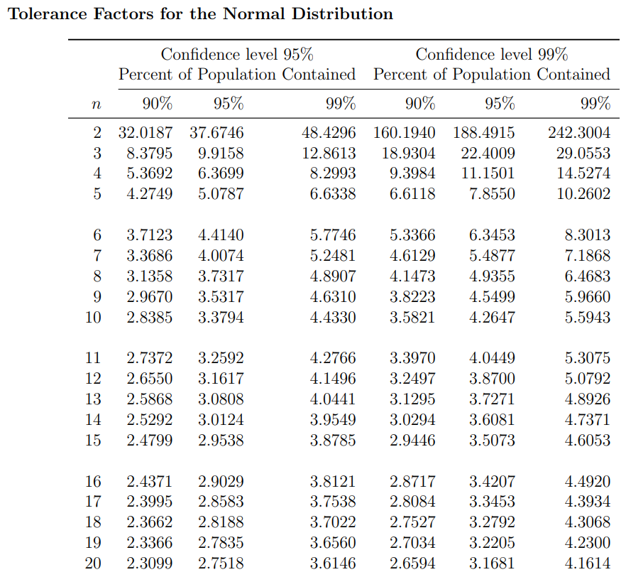
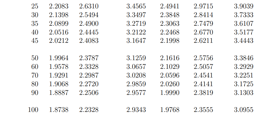
Tolerance Factors for the Normal Distribution
Confidence level 95%
Confidence level 99%
Percent of Population Contained Percent of Population Contained
n
90%
95%
99%
90%
95%
99%
2 32.0187 37.6746
48.4296 160.1940 188.4915
242.3004
3
8.3795
9.9158
12.8613
18.9304
22.4009
29.0553
4
5.3692
6.3699
8.2993
9.3984
11.1501
14.5274
5
4.2749
5.0787
6.6338
6.6118
7.8550
10.2602
6
3.7123
4.4140
5.7746
5.3366
6.3453
8.3013
7
3.3686
4.0074
5.2481
4.6129
5.4877
7.1868
8
3.1358
3.7317
4.8907
4.1473
4.9355
6.4683
9
2.9670
3.5317
4.6310
3.8223
4.5499
5.9660
10
2.8385
3.3794
4.4330
3.5821
4.2647
5.5943
11
2.7372
3.2592
4.2766
3.3970
4.0449
5.3075
12
2.6550
3.1617
4.1496
3.2497
3.8700
5.0792
13
2.5868
3.0808
4.0441
3.1295
3.7271
4.8926
14
2.5292
3.0124
3.9549
3.0294
3.6081
4.7371
15
2.4799
2.9538
3.8785
2.9446
3.5073
4.6053
16
2.4371
2.9029
3.8121
2.8717
3.4207
4.4920
17
2.3995
2.8583
3.7538
2.8084
3.3453
4.3934
18
2.3662
2.8188
3.7022
2.7527
3.2792
4.3068
19
2.3366
2.7835
3.6560
2.7034
3.2205
4.2300
20
2.3099
2.7518
3.6146
2.6594
3.1681
4.1614
25
2.2083
2.6310
3.4565
2.4941
2.9715
3.9039
30
2.1398
2.5494
3.3497
2.3848
2.8414
3.7333
35
2.0899
2.4900
3.2719
2.3063
2.7479
3.6107
40
2.0516
2.4445
3.2122
2.2468
2.6770
3.5177
45
2.0212
2.4083
3.1647
2.1998
2.6211
3.4443
50
1.9964
2.3787
3.1259
2.1616
2.5756
3.3846
60
1.9578
2.3328
3.0657
2.1029
2.5057
3.2929
70
1.9291
2.2987
3.0208
2.0596
2.4541
3.2251
80
1.9068
2.2720
2.9859
2.0260
2.4141
3.1725
90
1.8887
2.2506
2.9577
1.9990
2.3819
3.1303
100
1.8738
2.2328
2.9343
1.9768
2.3555
3.0955
6
Critical Values of the F Distribution for α = 0.05
ν1
ν2
1
2
3
4
5
6
7
8
9
10
12
15
20
24
30
40
60
120
∞
1 161.45 199.50 215.71 224.58 230.16 233.99 236.77 238.88 240.54 241.88 243.91 245.95 248.01 249.05 250.10 251.14 252.20 253.25 254.31
2
18.51
19.00
19.16
19.25
19.30
19.33
19.35
19.37
19.38
19.40
19.41
19.43
19.45
19.45
19.46
19.47
19.48
19.49
19.50
3
10.13
9.55
9.28
9.12
9.01
8.94
8.89
8.85
8.81
8.79
8.74
8.70
8.66
8.64
8.62
8.59
8.57
8.55
8.53
4
7.71
6.94
6.59
6.39
6.26
6.16
6.09
6.04
6.00
5.96
5.91
5.86
5.80
5.77
5.75
5.72
5.69
5.66
5.63
5
6.61
5.79
5.41
5.19
5.05
4.95
4.88
4.82
4.77
4.74
4.68
4.62
4.56
4.53
4.50
4.46
4.43
4.40
4.37
6
5.99
5.14
4.76
4.53
4.39
4.28
4.21
4.15
4.10
4.06
4.00
3.94
3.87
3.84
3.81
3.77
3.74
3.70
3.67
7
5.59
4.74
4.35
4.12
3.97
3.87
3.79
3.73
3.68
3.64
3.57
3.51
3.44
3.41
3.38
3.34
3.30
3.27
3.23
8
5.32
4.46
4.07
3.84
3.69
3.58
3.50
3.44
3.39
3.35
3.28
3.22
3.15
3.12
3.08
3.04
3.01
2.97
2.93
9
5.12
4.26
3.86
3.63
3.48
3.37
3.29
3.23
3.18
3.14
3.07
3.01
2.94
2.90
2.86
2.83
2.79
2.75
2.71
10
4.96
4.10
3.71
3.48
3.33
3.22
3.14
3.07
3.02
2.98
2.91
2.85
2.77
2.74
2.70
2.66
2.62
2.58
2.54
12
4.75
3.89
3.49
3.26
3.11
3.00
2.91
2.85
2.80
2.75
2.69
2.62
2.54
2.51
2.47
2.43
2.38
2.34
2.30
15
4.54
3.68
3.29
3.06
2.90
2.79
2.71
2.64
2.59
2.54
2.48
2.40
2.33
2.29
2.25
2.20
2.16
2.11
2.07
20
4.35
3.49
3.10
2.87
2.71
2.60
2.51
2.45
2.39
2.35
2.28
2.20
2.12
2.08
2.04
1.99
1.95
1.90
1.84
24
4.26
3.40
3.01
2.78
2.62
2.51
2.42
2.36
2.30
2.25
2.18
2.11
2.03
1.98
1.94
1.89
1.84
1.79
1.73
30
4.17
3.32
2.92
2.69
2.53
2.42
2.33
2.27
2.21
2.16
2.09
2.01
1.93
1.89
1.84
1.79
1.74
1.68
1.62
40
4.08
3.23
2.84
2.61
2.45
2.34
2.25
2.18
2.12
2.08
2.00
1.92
1.84
1.79
1.74
1.69
1.64
1.58
1.51
60
4.00
3.15
2.76
2.53
2.37
2.25
2.17
2.10
2.04
1.99
1.92
1.84
1.75
1.70
1.65
1.59
1.53
1.47
1.39
120
3.92
3.07
2.68
2.45
2.29
2.18
2.09
2.02
1.96
1.91
1.83
1.75
1.66
1.61
1.55
1.50
1.43
1.35
1.25
∞
3.84
3.00
2.60
2.37
2.21
2.10
2.01
1.94
1.88
1.83
1.75
1.67
1.57
1.52
1.46
1.39
1.32
1.22
1.00
Critical Values of the F Distribution for α = 0.01
ν1
ν2
1
2
3
4
5
6
7
8
9
10
12
15
20
24
30
40
60
120
∞
1 4052.18 4999.50 5403.35 5624.58 5763.65 5858.99 5928.36 5981.07 6022.47 6055.85 6106.32 6157.28 6208.73 6234.63 6260.65 6286.78 6313.03 6339.39 6365.86
2
98.50
99.00
99.17
99.25
99.30
99.33
99.36
99.37
99.39
99.40
99.42
99.43
99.45
99.46
99.47
99.47
99.48
99.49
99.50
3
34.12
30.82
29.46
28.71
28.24
27.91
27.67
27.49
27.35
27.23
27.05
26.87
26.69
26.60
26.50
26.41
26.32
26.22
26.13
4
21.20
18.00
16.69
15.98
15.52
15.21
14.98
14.80
14.66
14.55
14.37
14.20
14.02
13.93
13.84
13.75
13.65
13.56
13.46
5
16.26
13.27
12.06
11.39
10.97
10.67
10.46
10.29
10.16
10.05
9.89
9.72
9.55
9.47
9.38
9.29
9.20
9.11
9.02
6
13.75
10.92
9.78
9.15
8.75
8.47
8.26
8.10
7.98
7.87
7.72
7.56
7.40
7.31
7.23
7.14
7.06
6.97
6.88
7
12.25
9.55
8.45
7.85
7.46
7.19
6.99
6.84
6.72
6.62
6.47
6.31
6.16
6.07
5.99
5.91
5.82
5.74
5.65
8
11.26
8.65
7.59
7.01
6.63
6.37
6.18
6.03
5.91
5.81
5.67
5.52
5.36
5.28
5.20
5.12
5.03
4.95
4.86
9
10.56
8.02
6.99
6.42
6.06
5.80
5.61
5.47
5.35
5.26
5.11
4.96
4.81
4.73
4.65
4.57
4.48
4.40
4.31
10
10.04
7.56
6.55
5.99
5.64
5.39
5.20
5.06
4.94
4.85
4.71
4.56
4.41
4.33
4.25
4.17
4.08
4.00
3.91
12
9.33
6.93
5.95
5.41
5.06
4.82
4.64
4.50
4.39
4.30
4.16
4.01
3.86
3.78
3.70
3.62
3.54
3.45
3.36
15
8.68
6.36
5.42
4.89
4.56
4.32
4.14
4.00
3.89
3.80
3.67
3.52
3.37
3.29
3.21
3.13
3.05
2.96
2.87
20
8.10
5.85
4.94
4.43
4.10
3.87
3.70
3.56
3.46
3.37
3.23
3.09
2.94
2.86
2.78
2.69
2.61
2.52
2.42
24
7.82
5.61
4.72
4.22
3.90
3.67
3.50
3.36
3.26
3.17
3.03
2.89
2.74
2.66
2.58
2.49
2.40
2.31
2.21
30
7.56
5.39
4.51
4.02
3.70
3.47
3.30
3.17
3.07
2.98
2.84
2.70
2.55
2.47
2.39
2.30
2.21
2.11
2.01
40
7.31
5.18
4.31
3.83
3.51
3.29
3.12
2.99
2.89
2.80
2.66
2.52
2.37
2.29
2.20
2.11
2.02
1.92
1.80
60
7.08
4.98
4.13
3.65
3.34
3.12
2.95
2.82
2.72
2.63
2.50
2.35
2.20
2.12
2.03
1.94
1.84
1.73
1.60
120
6.85
4.79
3.95
3.48
3.17
2.96
2.79
2.66
2.56
2.47
2.34
2.19
2.03
1.95
1.86
1.76
1.66
1.53
1.38
∞
6.63
4.61
3.78
3.32
3.02
2.80
2.64
2.51
2.41
2.32
2.18
2.04
1.88
1.79
1.70
1.59
1.47
1.32
1.00
7
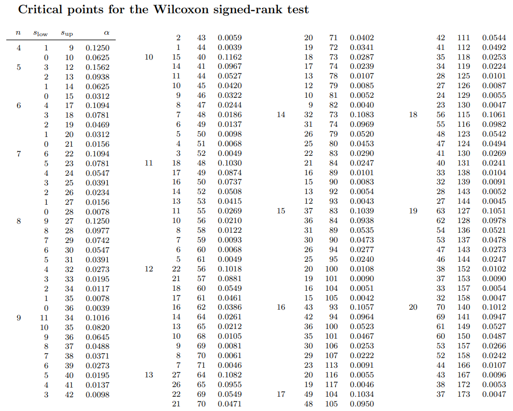
Critical points for the Wilcoxon signed-rank test
n
slow
sup
α
2
43
0.0059
20
71
0.0402
42
111
0.0544
4
1
9
0.1250
1
44
0.0039
19
72
0.0341
41
112
0.0492
0
10
0.0625
10
15
40
0.1162
18
73
0.0287
35
118
0.0253
5
3
12
0.1562
14
41
0.0967
17
74
0.0239
34
119
0.0224
2
13
0.0938
11
44
0.0527
13
78
0.0107
28
125
0.0101
1
14
0.0625
10
45
0.0420
12
79
0.0085
27
126
0.0087
0
15
0.0312
9
46
0.0322
10
81
0.0052
24
129
0.0055
6
4
17
0.1094
8
47
0.0244
9
82
0.0040
23
130
0.0047
3
18
0.0781
7
48
0.0186
14
32
73
0.1083
18
56
115
0.1061
2
19
0.0469
6
49
0.0137
31
74
0.0969
55
116
0.0982
1
20
0.0312
5
50
0.0098
26
79
0.0520
48
123
0.0542
0
21
0.0156
4
51
0.0068
25
80
0.0453
47
124
0.0494
7
6
22
0.1094
3
52
0.0049
22
83
0.0290
41
130
0.0269
5
23
0.0781
11
18
48
0.1030
21
84
0.0247
40
131
0.0241
4
24
0.0547
17
49
0.0874
16
89
0.0101
33
138
0.0104
3
25
0.0391
16
50
0.0737
15
90
0.0083
32
139
0.0091
2
26
0.0234
14
52
0.0508
13
92
0.0054
28
143
0.0052
1
27
0.0156
13
53
0.0415
12
93
0.0043
27
144
0.0045
0
28
0.0078
11
55
0.0269
15
37
83
0.1039
19
63
127
0.1051
8
9
27
0.1250
10
56
0.0210
36
84
0.0938
62
128
0.0978
8
28
0.0977
8
58
0.0122
31
89
0.0535
54
136
0.0521
7
29
0.0742
7
59
0.0093
30
90
0.0473
53
137
0.0478
6
30
0.0547
6
60
0.0068
26
94
0.0277
47
143
0.0273
5
31
0.0391
5
61
0.0049
25
95
0.0240
46
144
0.0247
4
32
0.0273
12
22
56
0.1018
20
100
0.0108
38
152
0.0102
3
33
0.0195
21
57
0.0881
19
101
0.0090
37
153
0.0090
2
34
0.0117
18
60
0.0549
16
104
0.0051
33
157
0.0054
1
35
0.0078
17
61
0.0461
15
105
0.0042
32
158
0.0047
0
36
0.0039
16
62
0.0386
16
43
93
0.1057
20
70
140
0.1012
9
11
34
0.1016
14
64
0.0261
42
94
0.0964
69
141
0.0947
10
35
0.0820
13
65
0.0212
36
100
0.0523
61
149
0.0527
9
36
0.0645
10
68
0.0105
35
101
0.0467
60
150
0.0487
8
37
0.0488
9
69
0.0081
30
106
0.0253
53
157
0.0266
7
38
0.0371
8
70
0.0061
29
107
0.0222
52
158
0.0242
6
39
0.0273
7
71
0.0046
23
113
0.0091
44
166
0.0107
5
40
0.0195
13
27
64
0.1082
20
116
0.0055
43
167
0.0096
4
41
0.0137
26
65
0.0955
19
117
0.0046
38
172
0.0053
3
42
0.0098
22
69
0.0549
17
49
104
0.1034
37
173
0.0047
21
70
0.0471
48
105
0.0950
9
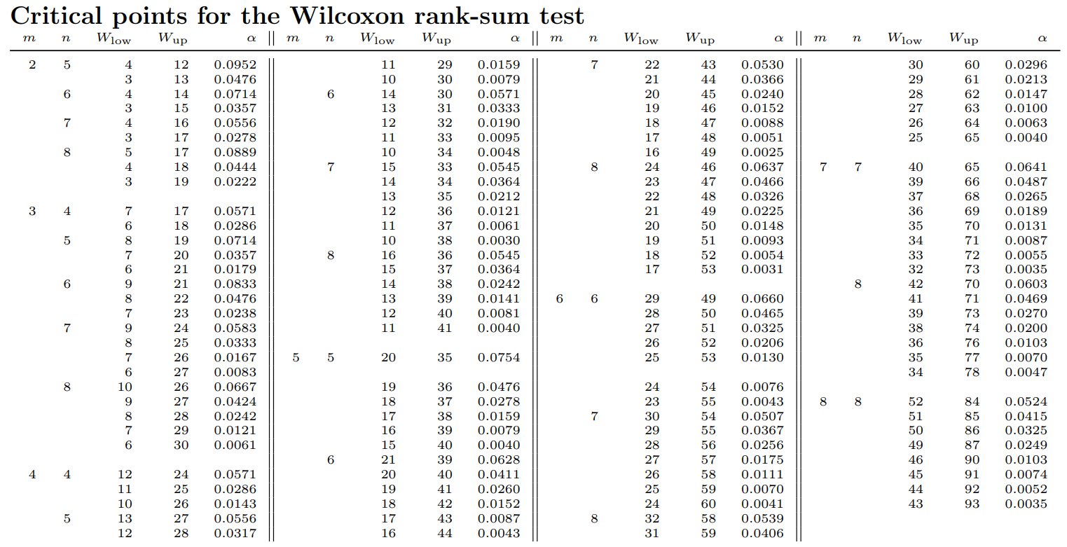
Critical points for the Wilcoxon rank-sum test
m
n
Wlow
Wup
α
m
n
Wlow
Wup
α
m
n
Wlow
Wup
α
m
n
Wlow
Wup
α
2
5
4
12
0.0952
11
29
0.0159
7
22
43
0.0530
30
60
0.0296
3
13
0.0476
10
30
0.0079
21
44
0.0366
29
61
0.0213
6
4
14
0.0714
6
14
30
0.0571
20
45
0.0240
28
62
0.0147
3
15
0.0357
13
31
0.0333
19
46
0.0152
27
63
0.0100
7
4
16
0.0556
12
32
0.0190
18
47
0.0088
26
64
0.0063
3
17
0.0278
11
33
0.0095
17
48
0.0051
25
65
0.0040
8
5
17
0.0889
10
34
0.0048
16
49
0.0025
4
18
0.0444
7
15
33
0.0545
8
24
46
0.0637
7
7
40
65
0.0641
3
19
0.0222
14
34
0.0364
23
47
0.0466
39
66
0.0487
13
35
0.0212
22
48
0.0326
37
68
0.0265
3
4
7
17
0.0571
12
36
0.0121
21
49
0.0225
36
69
0.0189
6
18
0.0286
11
37
0.0061
20
50
0.0148
35
70
0.0131
5
8
19
0.0714
10
38
0.0030
19
51
0.0093
34
71
0.0087
7
20
0.0357
8
16
36
0.0545
18
52
0.0054
33
72
0.0055
6
21
0.0179
15
37
0.0364
17
53
0.0031
32
73
0.0035
6
9
21
0.0833
14
38
0.0242
8
42
70
0.0603
8
22
0.0476
13
39
0.0141
6
6
29
49
0.0660
41
71
0.0469
7
23
0.0238
12
40
0.0081
28
50
0.0465
39
73
0.0270
7
9
24
0.0583
11
41
0.0040
27
51
0.0325
38
74
0.0200
8
25
0.0333
26
52
0.0206
36
76
0.0103
7
26
0.0167
5
5
20
35
0.0754
25
53
0.0130
35
77
0.0070
6
27
0.0083
34
78
0.0047
8
10
26
0.0667
19
36
0.0476
24
54
0.0076
9
27
0.0424
18
37
0.0278
23
55
0.0043
8
8
52
84
0.0524
8
28
0.0242
17
38
0.0159
7
30
54
0.0507
51
85
0.0415
7
29
0.0121
16
39
0.0079
29
55
0.0367
50
86
0.0325
6
30
0.0061
15
40
0.0040
28
56
0.0256
49
87
0.0249
6
21
39
0.0628
27
57
0.0175
46
90
0.0103
4
4
12
24
0.0571
20
40
0.0411
26
58
0.0111
45
91
0.0074
11
25
0.0286
19
41
0.0260
25
59
0.0070
44
92
0.0052
10
26
0.0143
18
42
0.0152
24
60
0.0041
43
93
0.0035
5
13
27
0.0556
17
43
0.0087
8
32
58
0.0539
12
28
0.0317
16
44
0.0043
31
59
0.0406
10
Critical Values of the Studentised Range Distribution for α = 0.05
ν1
ν2
2
3
4
5
6
7
8
9
10
11
12
13
14
15
16
17
18
19
20
2 6.0849 8.3308 9.7980 10.8810 11.7340 12.4345 13.0266 13.5381 13.9875 14.3874 14.7473 15.0757 15.3748 15.6503 15.9054 16.1427 16.3646 16.5728 16.7688
3 4.5007 5.9096 6.8245
7.5016
8.0370
8.4780
8.8521
9.1766
9.4620
9.7166
9.9460 10.1547 10.3459 10.5222 10.6856 10.8378 10.9803 11.1140 11.2400
4 3.9265 5.0403 5.7571
6.2870
6.7065
7.0528
7.3465
7.6015
7.8264
8.0271
8.2083
8.3732
8.5244
8.6640
8.7934
8.9141
9.0271
9.1332
9.2333
5 3.6354 4.6017 5.2185
5.6731
6.0329
6.3299
6.5823
6.8014
6.9947
7.1674
7.3237
7.4653
7.5956
7.7163
7.8280
7.9322
8.0298
8.1215
8.2080
6 3.4605 4.3390 4.8956
5.3049
5.6285
5.8953
6.1222
6.3192
6.4931
6.6485
6.7890
6.9169
7.0344
7.1428
7.2436
7.3375
7.4256
7.5086
7.5866
7 3.3439 4.1648 4.6812
5.0601
5.3591
5.6058
5.8154
5.9975
6.1581
6.3018
6.4314
6.5497
6.6583
6.7586
6.8518
6.9387
7.0202
7.0968
7.1691
8 3.2612 4.0410 4.5288
4.8858
5.1672
5.3991
5.5962
5.7673
5.9183
6.0534
6.1754
6.2867
6.3888
6.4832
6.5708
6.6527
6.7293
6.8015
6.8695
9 3.1991 3.9485 4.4149
4.7554
5.0235
5.2444
5.4319
5.5947
5.7384
5.8669
5.9830
6.0888
6.1860
6.2758
6.3592
6.4371
6.5101
6.5787
6.6435
10 3.1511 3.8768 4.3266
4.6543
4.9120
5.1242
5.3042
5.4605
5.5984
5.7217
5.8331
5.9346
6.0279
6.1141
6.1941
6.2689
6.3389
6.4048
6.4670
11 3.1127 3.8195 4.2561
4.5736
4.8229
5.0281
5.2021
5.3531
5.4863
5.6054
5.7129
5.8111
5.9012
5.9844
6.0617
6.1339
6.2015
6.2652
6.3252
12 3.0813 3.7728 4.1985
4.5076
4.7477
4.9469
5.1159
5.2625
5.3946
5.5102
5.6146
5.7098
5.7973
5.8781
5.9532
6.0231
6.0888
6.1506
6.2089
13 3.0553 3.7341 4.1509
4.4529
4.6897
4.8841
5.0490
5.1920
5.3181
5.4308
5.5326
5.6253
5.7105
5.7892
5.8623
5.9305
5.9945
6.0547
6.1116
14 3.0332 3.7014 4.1105
4.4066
4.6385
4.8290
4.9903
5.1300
5.2533
5.3635
5.4630
5.5537
5.6370
5.7139
5.7854
5.8521
5.9146
5.9735
6.0290
15 3.0143 3.6734 4.0760
4.3670
4.5947
4.7816
4.9399
5.0770
5.1979
5.3059
5.4033
5.4922
5.5738
5.6492
5.7193
5.7847
5.8459
5.9036
5.9580
16 2.9980 3.6491 4.0461
4.3327
4.5568
4.7406
4.8962
5.0310
5.1498
5.2559
5.3517
5.4390
5.5191
5.5931
5.6619
5.7261
5.7862
5.8429
5.8963
17 2.9837 3.6280 4.0200
4.3027
4.5237
4.7048
4.8580
4.9907
5.1077
5.2121
5.3064
5.3923
5.4712
5.5440
5.6117
5.6748
5.7339
5.7896
5.8421
18 2.9712 3.6093 3.9970
4.2763
4.4944
4.6731
4.8243
4.9552
5.0705
5.1735
5.2664
5.3511
5.4288
5.5006
5.5672
5.6295
5.6878
5.7426
5.7944
19 2.9600 3.5927 3.9766
4.2528
4.4685
4.6450
4.7944
4.9236
5.0375
5.1391
5.2308
5.3144
5.3911
5.4619
5.5277
5.5891
5.6466
5.7007
5.7518
20 2.9500 3.5779 3.9583
4.2319
4.4452
4.6199
4.7676
4.8954
5.0079
5.1083
5.1990
5.2815
5.3573
5.4273
5.4923
5.5529
5.6097
5.6632
5.7136
21 2.9410 3.5646 3.9419
4.2130
4.4244
4.5973
4.7435
4.8699
4.9813
5.0806
5.1703
5.2520
5.3269
5.3961
5.4603
5.5203
5.5765
5.6293
5.6792
22 2.9329 3.5526 3.9270
4.1959
4.4055
4.5769
4.7217
4.8469
4.9572
5.0556
5.1443
5.2252
5.2993
5.3678
5.4314
5.4908
5.5464
5.5987
5.6480
23 2.9255 3.5417 3.9136
4.1805
4.3883
4.5583
4.7019
4.8260
4.9353
5.0328
5.1207
5.2008
5.2743
5.3421
5.4051
5.4639
5.5189
5.5707
5.6196
24 2.9188 3.5317 3.9013
4.1663
4.3727
4.5413
4.6838
4.8069
4.9153
5.0119
5.0991
5.1785
5.2514
5.3186
5.3810
5.4393
5.4939
5.5452
5.5936
25 2.9126 3.5226 3.8900
4.1534
4.3583
4.5258
4.6672
4.7894
4.8969
4.9928
5.0793
5.1581
5.2303
5.2970
5.3590
5.4167
5.4709
5.5218
5.5698
30 2.8882 3.4865 3.8454
4.1021
4.3015
4.4642
4.6014
4.7199
4.8241
4.9170
5.0008
5.0770
5.1469
5.2114
5.2713
5.3271
5.3794
5.4286
5.4750
40 2.8583 3.4421 3.7907
4.0391
4.2317
4.3885
4.5205
4.6345
4.7345
4.8237
4.9039
4.9770
5.0439
5.1056
5.1629
5.2162
5.2662
5.3132
5.3575
60 2.8289 3.3987 3.7371
3.9774
4.1632
4.3142
4.4411
4.5504
4.6463
4.7317
4.8085
4.8783
4.9422
5.0011
5.0557
5.1066
5.1543
5.1990
5.2412
120 2.8000 3.3562 3.6846
3.9169
4.0960
4.2412
4.3630
4.4678
4.5596
4.6411
4.7144
4.7810
4.8418
4.8979
4.9499
4.9982
5.0435
5.0860
5.1260
Critical Values of the Studentised Range Distribution for α = 0.01
ν1
ν2
2
3
4
5
6
7
8
9
10
11
12
13
14
15
16
17
18
19
20
2 14.0346 19.0189 22.2935 24.7166 26.6280 28.1991 29.5282 30.6770 31.6866 32.5855 33.3946 34.1294 34.8018 35.4212 35.9948 36.5286 37.0277 37.4959 37.9368
3
8.2603 10.6157 12.1695 13.3241 14.2403 14.9972 15.6401 16.1978 16.6894 17.1283 17.5241 17.8844 18.2146 18.5192 18.8017 19.0650 19.3113 19.5427 19.7608
4
6.5113
8.1181
9.1729
9.9579 10.5823 11.0992 11.5394 11.9253 12.2639 12.5667 12.8403 13.0897 13.3186 13.5299 13.7262 13.9093 14.0808 14.2420 14.3940
5
5.7024
6.9757
7.8059
8.4215
8.9131
9.3208
9.6686
9.9713 10.2390 10.4787 10.6955 10.8932 11.0749 11.2428 11.3988 11.5445 11.6809 11.8093 11.9305
6
5.2427
6.3312
7.0333
7.5560
7.9737
8.3179
8.6113
8.8693
9.0966
9.3003
9.4847
9.6530
9.8077
9.9508 10.0838 10.2080 10.3245 10.4342 10.5377
7
4.9483
5.9193
6.5430
7.0061
7.3730
7.6784
7.9403
8.1672
8.3680
8.5478
8.7107
8.8593
8.9959
9.1242
9.2423
9.3526
9.4560
9.5534
9.6454
8
4.7445
5.6353
6.2039
6.6251
6.9600
7.2378
7.4748
7.6813
7.8642
8.0281
8.1766
8.3121
8.4368
8.5522
8.6595
8.7597
8.8538
8.9424
9.0260
9
4.5955
5.4279
5.9567
6.3473
6.6576
6.9148
7.1344
7.3257
7.4951
7.6470
7.7846
7.9103
8.0260
8.1330
8.2326
8.3257
8.4131
8.4953
8.5730
10
4.4818
5.2700
5.7686
6.1361
6.4276
6.6691
6.8751
7.0546
7.2136
7.3562
7.4854
7.6034
7.7120
7.8126
7.9062
7.9936
8.0757
8.1530
8.2261
11
4.3922
5.1459
5.6207
5.9701
6.2474
6.4759
6.6713
6.8415
6.9922
7.1274
7.2498
7.3617
7.4647
7.5600
7.6487
7.7317
7.8095
7.8829
7.9522
12
4.3197
5.0459
5.5016
5.8363
6.1011
6.3205
6.5069
6.6696
6.8136
6.9427
7.0597
7.1665
7.2649
7.3559
7.4407
7.5199
7.5943
7.6644
7.7306
13
4.2607
4.9635
5.4036
5.7266
5.9812
6.1919
6.3715
6.5283
6.6664
6.7905
6.9030
7.0057
7.1002
7.1877
7.2691
7.3453
7.4168
7.4841
7.5478
14
4.2099
4.8945
5.3215
5.6340
5.8808
6.0847
6.2583
6.4095
6.5428
6.6638
6.7716
6.8708
6.9621
7.0466
7.1252
7.1988
7.2678
7.3329
7.3943
15
4.1673
4.8359
5.2518
5.5558
5.7956
5.9936
6.1621
6.3087
6.4384
6.5547
6.6596
6.7568
6.8447
6.9266
7.0028
7.0741
7.1411
7.2041
7.2637
16
4.1306
4.7855
5.1919
5.4885
5.7223
5.9152
6.0793
6.2221
6.3483
6.4615
6.5639
6.6575
6.7431
6.8236
6.8975
6.9668
7.0319
7.0932
7.1512
17
4.0987
4.7417
5.1398
5.4300
5.6586
5.8471
6.0074
6.1468
6.2700
6.3804
6.4804
6.5717
6.6557
6.7334
6.8058
6.8734
6.9373
6.9974
7.0533
18
4.0707
4.7032
5.0941
5.3787
5.6027
5.7873
5.9443
6.0807
6.2013
6.3093
6.4071
6.4964
6.5785
6.6546
6.7253
6.7914
6.8535
6.9120
6.9673
19
4.0459
4.6693
5.0537
5.3334
5.5534
5.7345
5.8885
6.0223
6.1405
6.2464
6.3423
6.4298
6.5103
6.5848
6.6541
6.7189
6.7797
6.8370
6.8911
20
4.0237
4.6390
5.0178
5.2931
5.5094
5.6875
5.8388
5.9702
6.0864
6.1904
6.2845
6.3704
6.4494
6.5226
6.5906
6.6542
6.7139
6.7701
6.8232
21
4.0042
4.6119
4.9856
5.2569
5.4700
5.6453
5.7943
5.9236
6.0379
6.1402
6.2327
6.3172
6.3949
6.4668
6.5337
6.5962
6.6549
6.7101
6.7623
22
3.9864
4.5874
4.9565
5.2243
5.4345
5.6074
5.7541
5.8816
5.9941
6.0949
6.1860
6.2692
6.3457
6.4165
6.4823
6.5439
6.6016
6.6560
6.7074
23
3.9703
4.5653
4.9302
5.1948
5.4023
5.5729
5.7178
5.8435
5.9545
6.0538
6.1437
6.2257
6.3011
6.3709
6.4358
6.4964
6.5533
6.6070
6.6576
24
3.9557
4.5452
4.9063
5.1679
5.3730
5.5416
5.6847
5.8088
5.9184
6.0165
6.1052
6.1861
6.2605
6.3294
6.3934
6.4532
6.5094
6.5623
6.6122
25
3.9424
4.5268
4.8844
5.1433
5.3463
5.5130
5.6544
5.7771
5.8854
5.9823
6.0700
6.1499
6.2234
6.2914
6.3546
6.4137
6.4692
6.5214
6.5707
30
3.8891
4.4545
4.7992
5.0476
5.2418
5.4012
5.5361
5.6531
5.7563
5.8485
5.9318
6.0079
6.0777
6.1423
6.2023
6.2584
6.3105
6.3601
6.4069
40
3.8247
4.3671
4.6951
4.9308
5.1145
5.2649
5.3920
5.5020
5.5989
5.6855
5.7636
5.8348
5.9002
5.9606
6.0168
6.0692
6.1183
6.1646
6.2083
60
3.7622
4.2822
4.5942
4.8178
4.9913
5.1330
5.2525
5.3558
5.4466
5.5276
5.6007
5.6672
5.7282
5.7845
5.8368
5.8856
5.9313
5.9743
6.0149
120
3.7017
4.2000
4.4970
4.7085
4.8720
5.0055
5.1176
5.2143
5.2992
5.3748
5.4429
5.5048
5.5615
5.6138
5.6623
5.7075
5.7499
5.7897
5.8272
11
Student ID: . . . . . . . . . . . . . . . . . . . . . . .
* * * * * * * * * * * * * * *
EEEN 320
Page
17 of
17
 Final Examination 2023
EEEN320
Signals, Systems and Statistics 2
Time allowed: One Hour
Total number of questions: 3
Total marks: 100 marks
Instructions:
Answer all questions.
Write your name and student ID on each page of
Final Examination 2023
EEEN320
Signals, Systems and Statistics 2
Time allowed: One Hour
Total number of questions: 3
Total marks: 100 marks
Instructions:
Answer all questions.
Write your name and student ID on each page of
the answer papers.
Clearly label the question numbers and the
corresponding parts of the questions.
To get a full score you must write or type your
answers neatly, showing your solution steps and
reasoning clearly.
Calculator permitted.
(Blank page)
Q1 Small Sample Hypothesis Test for a Population Mean [20 marks]
In a university postgraduate entrance examination, students are required to take tests
consisting of randomly selected multiple-choice questions six times. This rigorous
practice ensures that students have a solid understanding of the material. The
university acceptance standard mandates that the average test score must exceed 85%
(out of 100%). To evaluate a random student's performance, they were selected to
take the six tests, and their scores, represented in percentages, are as follows:
93.2 87.0 92.1 90.1 87.3 93.6
A hypothesis test will be done to determine whether to accept the student or not.
a) State the appropriate null and alternate hypotheses.
[5 marks]
b) Clearly demonstrate the process of determining the P-value. Note: You may
compute an exact value or provide a sensible justification to obtain the most
probable value, which is also acceptable.
[10 marks]
c) Should the student be accepted? Explain.
[5 marks]
Q2 Wilcoxon Rank-Sum Test [20 marks]
A person living in Johnsonville is trying to determine which of the two bus routes
arriving at Wellington Station has a shorter commute time. Times in minutes for six
trips on bus route No. 1 and five trips on bus route No. 22 are as follows:
Bus Route No. 1:
16.0 15.7 16.4 15.9 16.2 16.3
Bus Route No. 22:
17.2 16.9 16.1 19.8 16.7
Can you conclude that the mean commute time is less for bus route No. 1?
Q3. Uncertainties in the Least-Squares Coefficients [60 marks]
The coefficient of learning (COL) for a student is a measure of how well they can
remember what they have studied. The following measurements of the COL and the
learning time (in hours) for seven students have been collected. The results are
presented in the following table:
Learning time
COL
1.750
0.80
1.632
0.78
1.594
0.77
1.623
0.75
1.495
0.71
1.465
0.66
1.272
0.63
a) Compute the least-squares line for predicting COL from learning time.
[10 marks]
b) Compute the error standard deviation estimate
s.
[10 marks]
c) Compute a 95% confidence interval for the slope.
[10 marks]
d) Find a 95% confidence interval for the mean COL for students with learning
time of 1.5 hours.
[10 marks]
e) Can you conclude that the mean COL for students with learning time of 1.5
hours is less than 0.75? Perform a hypothesis test and report the P-value.
Note: you can either compute an exact value; or a sensible justification to obtain
the most probable value is also sufficient.
[10 marks]
f) Find a 95% prediction interval for the COL of a particular student whose
learning time is 1.5 hours.
[10 marks]
~~ End of Examinations ~~
 EXAMINATIONS – 2024
TRIMESTER 2
FRONT PAGE
EEEN320
SIGNALS, SYSTEMS AND STATISTICS 2
16/08/2024
Time allowed:
EXAMINATIONS – 2024
TRIMESTER 2
FRONT PAGE
EEEN320
SIGNALS, SYSTEMS AND STATISTICS 2
16/08/2024
Time allowed: TWO HOURS (2pm – 4pm)
Instructions:
Answer all 4 questions.
Marks allocations are as indicated at the end of each question.
Closed book.
Only silent non-programmable calculators or silent programmable calculators
with their memories cleared are permitted in this examination.
Statistical tables are provided at the end of the question scripts.
You are allowed to bring in a two-page A4-sized of notes and formulae.
Write all the solutions, including working steps, in the answer scripts. Label
each question clearly. Nothing on this question booklet will be marked.
Write your name and student ID on the answer scripts clearly.
EEEN320
Page
1 of
9
1. Confidence Interval (for the difference between two proportions) [20 marks]
Meal delivery companies usually promise on-time delivery, e.g. your order will be delivered in 10
minutes otherwise your money will be returned. A survey of two meal delivery companies,
“Hungry?” and “Cuisine”, was carried out. It was reported that out of 1985 deliveries completed by
“Hungry?”, 1919 were on-time, and for “Cuisine” 4561 out of 4988 were on-time.
a) Calculate the proportion of on-time deliveries for each of the delivery company. [6 marks]
b) Calculate the standard deviation of on-time deliveries for each of the delivery company.
[6 marks]
c) Find a 99% confidence interval for the difference between the proportion of on-time deliveries
for the two companies.
[8 marks]
2. Hypothesis Testing (small sample test for the difference between two means) [20 marks]
Buses tend to run late during peak hours. A new on-time arrival process is being contemplated.
Measurements of the lateness (in minutes) of random buses arriving at the same bus terminal using
the old and new arrival process produced the following data:
Old (
X): 16.3 15.9 15.8 16.2 16.1 16.0 15.7 15.8 15.9 16.1 16.3 16.1 15.8 15.7 15.8 15.7
New (
Y): 15.9 16.2 16.0 15.8 16.1 16.1 15.8 16.0 16.2 15.9 15.7 16.2 15.8 15.8 16.2 16.3
a) Calculate the mean for each of the old and new method.
[5 marks]
b) Calculate the standard deviation for each of the old and new method.
[5 marks]
c) The bus company is interested to answer the question “Can you conclude at the 5% level that
one process yields a different mean lateness than the other?”
Set up a hypothesis testing to help answer the question. Show your working steps and your
conclusion clearly.
[10 marks]
Note: you do not need to calculate the exact
P-value, as it is sufficient to provide a logical
approximation (and explain the justification).
3. Wilcoxon Rank-Sum Test [20 marks]
A person is trying to determine which of the two bus routes arriving at Wellington Station has a
shorter commute time. Times in minutes for five trips on bus route A and six trips on bus route B are
as follows:
Bus Route A (
X):
17.2 16.9 16.1 19.8 16.7
Bus Route B (
Y):
16.0 15.7 16.4 15.9 16.2 16.3
Can you conclude that the mean commute time is less for bus route B?
EEEN320
Page
2 of
9
4. Uncertainties in the Least-Squares Coefficients [40 marks]
The coefficient of learning (COL) for a student is a measure of how well they can remember what
they have studied. The following measurements of the COL and the learning time (in hours) for seven
students have been collected. The results are presented in the following table:
Learning time, 𝒙
COL, 𝒚
1.750
0.80
1.632
0.78
1.594
0.77
1.623
0.75
1.495
0.71
1.465
0.66
1.272
0.63
You can use the following quantities provided: ∑𝑛 (𝑥
𝑛
𝑖=1
𝑖 − 𝑥̅)2 = 0.141471, ∑
(𝑦
𝑖=1
𝑖 − 𝑦
̅)2 =
0.0246857, ∑𝑛 (𝑥
𝑖=1
𝑖 − 𝑥̅)(𝑦𝑖 − 𝑦
̅) = 0.0561429.
a) Compute the least-squares line for predicting COL from learning time.
[10 marks]
b) Compute the error standard deviation estimate,
s.
[6 marks]
c) Compute a 95% confidence interval for the slope.
[7 marks]
d) Find a 95% confidence interval for the mean COL for students with a learning time of 1.5
hours.
[7 marks]
e) Can you conclude that the mean COL for students with a learning time of 1.5 hours is less
than 0.75? Perform a hypothesis test and report the P-value.
Note: you do not need to compute an exact value; a sensible justification using the t-table to
obtain the most probable value is sufficient.
[10 marks]
********************
EEEN320
Page
3 of
9
EEEN320
Page
4 of
9
EEEN320
Page
5 of
9
 Chi-square distribution
EEEN320
Page
6 of
9
EEEN320
Page
7 of
9
EEEN320
Page
8 of
9
EEEN320
Page
9 of
9
 EXAMINATIONS – 2024
TRIMESTER 2
FRONT PAGE
EXAMINATIONS – 2024
TRIMESTER 2
FRONT PAGE
EEEN 320
SIGNALS, SYSTEMS AND STATISTICS 2
30/10/2024
Time allowed: TWO HOURS
Instructions:
Answer all four questions.
Each question has a maximum of 30 marks
Closed Book
Only silent non-programmable calculators or silent programmable calculators
with their memories cleared are permitted in this examination
A single sheet (double sided) of A4 paper with notes is permitted
EEEN320
Page
1 of
3
1. Interference Removal
(30 marks)
An analogue signal with a bandwidth of 1000 Hz is to be sampled for processing. The signal
contains a strong unwanted interference component at 2500 Hz that must be reduced by (at least) 50
dB if the system is to work correctly.
a)
Consider the case where an antialiasing filter is to be used to remove the interference
component.
i.
What would be the minimum required order for the filter?
[10 MARKS]
ii. What would be the gain of the resulting filter at 2500 Hz? (Assume unity gain in the passband.)
[5 MARKS]
iii. At what (minimum) frequency must the filtered signal be sampled?
[5 MARKS]
b) An alternative strategy would be to capture the signal including the interference component
and then use a digital filter to remove the intereference. At what (minimum) frequency must
the signal now be sampled?
[5 MARKS]
c) Discuss the relative merits of the two approaches.
[5 MARKS]
2. Analogue Filter Design
(30 marks)
A third order Chebychev type I low pass filter with its corner frequency at 1 rad/s and 0.5 dB of
passband ripple has transfer function
G(s) = 0.72 / [ (s + 0.6265) (s2 + 0.6265 s + 1.142) ] .
a) Sketch the frequency response (both gain and phase) of the filter, making sure to note any
prominent features of the response.
[10 MARKS]
b) Frequency scale the transfer function so that its corner frequency lies at 100 Hz.
[10 MARKS]
c)
Find the transfer function of the corresponding high pass filter, again with its corner frequency
at 100 Hz.
[10 MARKS]
EEEN320
Page
2 of
3
3. Spectral Estimation
(30 marks)
You wish to use the Fourier transform to distinguish between two pure sine waves at 432 Hz and
440 Hz that may be present in a signal.
a) What is the minimum sampling frequency that you would use when collecting the data to
avoid aliasing?
[5 MARKS]
b) How many data points must you collect if the DFT is to be able to distinguish between the two
frequencies?
[5 MARKS]
c) Would you use a window function when collecting the data? Explain why or why not.
[5 MARKS]
d) If you were to use a window, describe the resulting effect on the spectrum obtained, as well as
any changes you would make to your data collection choices.
[5 MARKS]
e) If the system were configured so that its Nyquist frequency was 200 Hz, would it still be
possible to distinguish between the two input frequencies?
[5 MARKS]
f)
Is there any sampling frequency that would cause the two input frequencies to appear
equal? If so find such a frequency.
[5 MARKS]
4.
Finite Impulse Response Filters
(30 marks)
A low-pass, FIR filter of 51st order is designed using a Hann window. Describe with appropriate
diagrams how the filter response would change if
a)
The order of the filter were reduced to 31st order,
[10 MARKS]
b) The Hann window were replaced with a Blackman window,
[10 MARKS]
c)
The sinc function used in the design were made twice as wide.
[10 MARKS]
********************
EEEN320
Page
3 of
3
Document Outline