Tahr grazing Potential of Tier 1 and alternative monitoring networks Manaaki Whenua 2018.pdf

Potential of Tier One and alternative
monitoring networks to assess the
ecological integrity of alpine vegetation
exposed to tahr grazing

Prepared for:
DOC
October 2018

Potential of Tier One and alternative monitoring networks
to assess the ecological integrity of alpine vegetation
exposed to tahr grazing
Contract Report: LC3328

Peter Bellingham, Susan Wiser, Olivia Burge, Tomás Easdale, Sarah Richardson
Manaaki Whenua – Landcare Research

Reviewed by:
Approved for release by:
William Lee
Gary Houliston
Senior Researcher
Portfolio Leader – Enhancing Biodiversity
Manaaki Whenua – Landcare Research
Manaaki Whenua – Landcare Research

© Department of Conservation 2018
This report has been produced by Landcare Research New Zealand Ltd for the New Zealand Department of
Conservation. All copyright in this report is the property of the Crown and any unauthorised publication,
reproduction, or adaptation of this report is a breach of that copyright and illegal.
- i -

Summary
Objectives and Client
•
The goal of this report was to evaluate the statistical and ecological power of grid-based
Tier 1 data to report on ecological integrity in alpine regions between two management
areas designated for Himalayan tahr (i.e. the tahr management and exclusion zones), and
to review the potential to integrate Tier 1 monitoring with 117 pre-existing, subjectively
located vegetation plots designed to report on tahr impacts. This was achieved by
comparing the physical environments, animal distributions, and vegetation composition
across the three groups of plots (i.e. Tier 1 plots in the management zone, subjectively
located plots in the management zone, and Tier 1 plots in the exclusion zone), and
assessing the distribution and capacity to report change of selected indicator plant taxa.
The work was undertaken for the Department of Conservation between August 2017 and
August 2018.
Methods
•
We used environmental, vegetation, and animal distribution and pellet data from three
plot groups: Tier 1 plots in the tahr management zone; Tier 1 plots in the tahr exclusion
zone; and subjectively located plots in the tahr management zone.
•
We used linear models using environmental covariates to evaluate the comparability of
the three plot groups. Elevation, aspect, latitude, slope and soil chemistry data came
from plot measurements; potential solar radiation was computed; and modelled climate
variables came from interpolated surfaces.
•
We intersected plot locations with pest distribution polygons supplied by DOC and used
general linear models to compare the frequency of non-native terrestrial vertebrate
species across the three plot groups. We used generalised binomial models to compare
ungulate and lagomorph pellet frequency across the three plot groups.
•
We compared vegetation composition across the three plot groups by classifying
vegetation on each plot according to existing woody and non-woody vegetation
classifications. We also used non-metric multidimensional scaling ordination to visualise
and describe key compositional gradients.
•
We reviewed the vegetation indicators currently used to detect tahr impacts. We
compared the frequencies of each indicator species across the three plot groups;
summarised the environments where each species is found; tested for concordance
between two methods for measuring tussock condition; and conducted statistical power
analyses to determine the effect sizes that can be detected over time.
•
We used propensity scoring models to test whether a suite of tahr impact indicators
differed between the tahr management and tahr exclusion zones. This approach used
covariate data to ‘match’ plots in the two treatments.
Results
•
Tier 1 management zone plots had significantly higher elevations and hence colder mean
annual temperatures than the Tier 1 exclusion zone plots. The subjectively located plots
had significantly higher mean annual temperatures than the Tier 1 management zone
- v -

plots despite their elevations not being significantly lower. Most moisture-related
variables and solar radiation were not significantly different between the Tier 1
management and exclusion zone plots, with the exception of lower air humidity and
lower sunshine hours in the Tier 1 management zone plots. Subjectively located plots
occurred on wetter sites with lower solar radiation than the Tier 1 plots in the
management zone. Mineral soil pH was lower in the Tier 1 exclusion zone plots than
those in the management zone but total phosphorus concentrations were similar.
•
Eight pest species differed in their distribution between the subjectively located plots
and the Tier 1 management zone plots (ferret, hare, hedgehog, possum, red deer, ship
rat, stoat, weasel). Ten pest species differed in their distribution between the Tier 1
management zone and exclusion zone plots (cat, ferret, hare, hedgehog, mouse, Norway
rat, possum, red deer, ship rat, weasel). Ungulate pellets occurred more frequently in the
Tier 1 management zone plots than in the Tier 1 exclusion zone plots. Ungulate pellets
were ca. 8 times more frequent in subjectively located plots than in Tier 1 management
zone plots. Hare pellet frequency was similar between the two Tier 1 zones but both
were significantly higher than the subjectively located plots.
•
At least one third of the vegetation plots in each group could not be assigned to a pre-
defined vegetation community, which limits the scope for comparing across the three
plots groups. However, of the plots that were assigned, 65% of the subjectively located
plots were non-woody, compared with 24% of the Tier 1 plots in the management zone,
and 19% of the Tier 1 plots in the exclusion zone. Conversely, 38% of the aligned Tier 1
plots in the exclusion zone were woody, compared with just 15% of the Tier 1 plots in the
management zone and < 1% in the subjectively located plots. Over half of the assigned
subjectively located plots were assigned to a Chionochloa pallens community that only
occurred once in the Tier 1 plots. A 3-axis ordination revealed very high compositional
turnover across the three plot groups spanning high alpine rocky fellfields, dry
intermontane shrublands, and tall rain forest communities. This turnover underpins the
significant challenge for deriving consistent indicators of tahr impacts across very diverse
ecosystems. Tier 1 management zone plots sampled a wide range of alpine
environments, Tier 1 exclusion zone plots included forest vegetation and the subjectively
located plots sampled a narrow range of compositional variation.
•
The frequencies of 12 palatable plant species used as indicators were statistically similar
between the two Tier 1 plot groups. The frequency of Chionochloa pallens was much
greater in the subjectively located plots than in Tier 1 plots in both the management and
exclusion zones, while C. flavescens was twice as frequent in Tier 1 plots in the exclusion
zone as in the management zone (both Tier 1 and subjectively located plots). In the
management zone, Aciphylla divisa was four time more frequent in subjectively located
plots than in Tier 1 plots. The 12 indicator species split into 3 groups – low, medium and
high rainfall species. The basal area of tussocks was positively related to visual estimates
of crown cover at both the subplot and plot scales. The Tier 1 plot network has sufficient
statistical power to detect differences of tussock cover of ca. 20% and cover change of
ca. 23% over 5 years. There is low statistical power to detect differences in individual
species, particularly for uncommon (potentially more vulnerable) species, supporting the
case for additional Tier 2 monitoring.
•
Propensity scoring models detected evidence of lower shrub cover in the Tier 1
management zone plots, relative to the Tier 1 exclusion zone, but this should be
interpreted cautiously given the very low number of plots informing this analysis.
- vi -

Conclusions
•
The Tier 1 network provides the first objective sample of vegetation composition across
the alpine landscape at a national scale. These data are a significant scientific milestone
and a crucial first step for developing a robust monitoring programme for assessing tahr
impacts against other drivers of compositional variation in the alpine region.
•
Comparisons between Tier 1 plots and the subjectively located plots identified the extent
of environmental and compositional bias in the subjectively located plots. The latter were
designed to sample Chionochloa pallens grasslands, which are a small part of the
compositional variation sampled by Tier 1 plots.
•
Published accounts emphasise that tahr can diminish ecosystem function and alter the
structure of dominant grasses and shrubs in alpine grasslands and subalpine shrublands
respectively. However, these impacts can be highly concentrated at a patch scale (c. 300
m2), in which less palatable (usually native) low-stature plant species can become more
dominant. It is unknown whether such grazing-induced effects on ecological integrity are
reversible, and how they interact with effects of climate change. Quantifying these
impacts and recovery processes following tahr management will require integration of
Tier 1 data (to provide an unbiased sample of ‘background’ dynamics), with the existing
subjectively located plots (to provide valuable longitudinal data, albeit from subjectively
located plots in one vegetation type), alongside new Tier 2 monitoring sampling specific
catchments or vegetation communities using unbiased sampling methods, and new Tier
3 monitoring to understand the recovery of grazing-induced vegetation types. Such an
integrated, comprehensive monitoring programme will also deliver a richer
understanding of alpine vegetation dynamics. We lack the depth of understanding in the
alpine that we have from forested ecosystems and this limits our capacity to interpret
monitoring data and forecast likely changes.
•
We could strengthen our confidence in tahr impact assessments by quantifying dietary
preference indices for a full range of plant species. This would reveal defensible ways of
aggregating plant species for use as indicators on the basis of their palatability to tahr,
and could be done alongside new Tier 2 monitoring.
•
Rates and trajectories of recovery by grazing-induced vegetation types are unknown.
Slow or partial recovery could have severe, cumulative, degradative impacts on
vegetation integrity over time, if areas targeted by tahr fail to recover over timescales
matched by plant recruitment processes. Focused studies of highly impacted areas, with
experimental manipulations, would be ideal for Tier 3 research studies.
Recommendations
1  With respect to determining impacts of tahr on the ecological integrity of alpine and
subalpine ecosystems, we recommend:
a  continuing measurement of the subjectively located plots in tahr habitat
b  establishing a representative (Tier 2) vegetation plot network
c  instigating long-term studies as measurements of Tier 3 (research) plots.
2  With respect to methods on current plots, we recommend:
a  maintaining current additional measurements on Tier 1 plots
- vii -

b  using constant areas within Tier 1 plots to quantify Chionochloa spp.
c  evaluating the suitability of height frequency methods and distance-based tussock
measurements.
3  With respect to new research, we recommend:
a  determining the dietary preference of tahr
b  undertaking a study of hare diet and dietary preferences
c  establishing a ‘null model’ of ecological integrity in alpine and subalpine ecosystems.

- viii -

1
Introduction
Himalayan tahr (Hemitragus jemlahicus) were liberated at the Hermitage in Mount Cook
National Park in 1904 and 1909, from which a wild population established rapidly (Caughley
1970a; Forsyth & Tustin 2005). They expanded to occupy c. 6,150 km2 of the Southern Alps,
centred on the point of liberation, in the 1970s, which was reduced by aerial hunting to 4,259
km2 in 1996 (Forsyth & Tustin 2005). Within their range, tahr mostly occupy shrublands and
tussock grasslands above treeline, but move within season and among seasons to other
vegetation below treeline (Tustin & Parkes 1988). Tussocks (Chionochloa spp.) feature
prominently in the diet of tahr, especially in winter, while other grasses (Poa colensoi and
Rytidosperma setifolium) and sedges (e.g. Schoenus pauciflorus) are components of the diet
in summer (Tustin & Parkes 1988). Woody plants (notably Dracophyllum spp.) are also
important in their diet, as are several herbs (e.g. Celmisia spp., Aciphylla spp., Ranunculus
lyallii). Other mammalian herbivores, especially chamois (Rupicapra rupicapra), brown hares
(Lepus europaeus), and red deer (Cervus elaphus scoticus), occupy the same habitats as tahr
and consume many of the same native plant species.
The Himalayan Tahr Control Plan and the Tahr Management Policy (Department of
Conservation 1993) established a national tahr population limit of no more than 10,000
individuals within a tahr management zone in the central Southern Alps and defined
maximum tahr density thresholds within 11 management units in that zone. DOC established
a tahr exclusion zone, with a block to the north and a block to the south of the management
zone, which is managed with an aim of zero density of tahr. Within the management zone,
vegetation plots were established to monitor the impacts of tahr on sensitive subalpine
vegetation and to help guide management of tahr densities. But the historic sampling design
has limitations. Plots were subjectively located in areas of tussock grasslands and were of
variable size (with a requirement to monitor > 20 individual snow tussock plants). This limits
assessment and reporting to tussock grasslands at the catchment level but the Department
of Conservation now requires broader statements about the impact of tahr on vegetation
communities across the entire landscape where tahr occur (McKay & McNutt 2016). Tahr can
cause severe degradation to woody and herbaceous alpine vegetation (Wilson 1970) and
legacies of degradation from overgrazing or other effects can strongly influence
demographic processes and affect the capacity of degraded grasslands to recover in biomass
(Holdaway et al. 2014). However, tahr cause highly localised and severe degradation to
vegetation, with heavily grazed patches (c. 300 m2) sometimes immediately adjacent to
ungrazed patches (Wilson 1970). As a consequence, there is a need to evaluate ecological
integrity systematically in alpine regions with and without tahr.
The Department of Conservation needs to evaluate the extent to which tahr degrade the
ecological integrity of alpine and subalpine ecosystems. The current design is to compare the
ecological integrity of the tahr exclusion zone with that of the tahr management zone. The
goal of this report is to answer whether the two zones are comparable in environment, plant
communities, and the presence of co-occurring introduced mammals. DOC currently
measures structurally dominant plants (Chionochloa tussock species and subalpine shrubs)
and some plant species that are likely to be preferred by tahr and therefore potentially
vulnerable (Department of Conservation 1993; McKay & McNutt 2016). This report provides a
basis to determine whether future comparisons of vegetation between the tahr management
and exclusion zones are defensible, and makes recommendations for improving the capacity
- 1 -

to determine the extent to which tahr degrade the ecological integrity of alpine and
subalpine ecosystems.
2
Objectives
The goal of this report is to evaluate the statistical and ecological power of grid-based Tier 1
data to report on landscape-level ecological integrity in alpine regions according to two
management areas for Himalayan tahr (i.e. the tahr management and exclusion zones), and
to review the potential to integrate Tier 1 monitoring with monitoring from 117 pre-existing,
subjectively located vegetation plots designed to report on tahr impacts.
The analysis we present includes:
•
Environmental covariate matching. This analysis compared the environments represented
by the tahr management and exclusion zones into order to evaluate the defensibility of
comparisons between them. We used environmental covariate data from 3 datasets: Tier
1 plots from the tahr management zone; Tier 1 plots from the tahr exclusion zone; the
117 pre-existing vegetation plots designed to measure tahr impacts within the tahr
management zone. Environmental covariates analysed include elevation, aspect, latitude,
slope and soil chemistry data from plot measurements, where available, and potential
solar radiation as computed from plot measurements. Plot locations were intersected
with climate surfaces supplied by NIWA to obtain values for eight climate variables.
•
Co-occurring animals. This analysis used mapped distributions of other non-native
terrestrial vertebrate species (e.g. chamois, hare, possum, red deer), and pellet data from
lagomorphs to determine whether plots in the tahr management zone and the tahr
exclusion zone had similar abundances of co-occurring vertebrate herbivores. Where
suitable pellet data were available, this analysis included the 117 subjectively located
vegetation plots designed to measure tahr impacts.
•
Vegetation communities provide context for determining tahr impacts. We classified
each vegetation plot in the three datasets according to the woody (Wiser et al. 2011,
2013) and non-woody (Wiser et al. 2016) national plot-based vegetation classifications.
To complement this, we used ordination to visualise and describe the compositional
gradients across the three plot datasets.
•
We reviewed indicators currently measured on alpine vegetation plots to detect tahr
impacts (see McKay & McNutt (2016) Tier 1 Vegetation Monitoring – Tahr Browse
Impacts Protocol - DOC-2664865) for a description of the additional measurements
made on Tier 1 plots in the tahr management zone and tahr exclusion zone and the likely
indicators that can be reported on from those additional measurements, and the
standard Tier 1 measurements). This involved:
•
A review of the ecological value of the plant indicator species selected by DOC
(McKay & McNutt 2016) that are used to determine tahr impacts. We summarised
the environments where adult plants of these species are found (e.g. snowbank
specialists, subalpine generalists) and related these environments to habitat-use by
tahr to assess their broader utility for comparisons between the tahr management
and exclusion zones.
- 2 -

•
A review of whether additional measurements are required to derive useful
indicators of tahr impacts on Tier 1 plots in the tahr management and exclusion
zones.
•
A statistical power analysis to determine the effect sizes of tahr-impact indicators
that can be detected over time. As re-measurement data are lacking for the new
methods being used on Tier 1 plots in the tahr management zone and tahr exclusion
zone (see Tier 1 Vegetation Monitoring – Tahr Browse Impacts Protocol – DOC-
2664865), we simulated a range of possible changes in each indicator at the plot-
level.
•
The use of propensity scoring models to test whether a suite of tahr impact indicators
differed between the tahr management and tahr exclusion zones. This approach used
covariate data to ‘match’ plots in the two treatments. This analysis built on the analyses
of environmental covariates in (a) and the biological covariates for animals in (b).
The original contract additionally includes an analysis testing whether the current
subsampling method used on Tier 1 plots (i.e. measuring individual tussocks in a subset of 5
m × 5 m subplots) is statistically robust for estimating plot-level tussock condition. By
agreement with DOC, this analysis was not completed because there were too few plots
where all subplots had been measured. Without such data, it was not possible to assess
whether subsampling by subplot yields a satisfactory estimate of plot-level tussock cover.
3
Datasets
3.1  Identifying Tier 1 plots within the tahr management zone and tahr
exclusion zone
Tier 1 samples locations at the intersections of a national 8 km grid. We used a data set
supplied by DOC that identified extant Tier 1 sample point locations where a vegetation plot
has been sampled (‘EntireGridWithConsUnitsAndOverlyingDOCLand_07May2013.xls’) and
intersected these data with the spatial layer of the tahr management zone and tahr exclusion
zone provided by DOC (layer ‘Tahr_Mgt_Units_1993’ in the geodatabase
‘TahrMonitoringLCR_data.gdb’ (“the management layer”). This gave us the subset of Tier 1
locations that fell within the exclusion or management zones (Fig. 1).
- 3 -

link to page 14 link to page 15

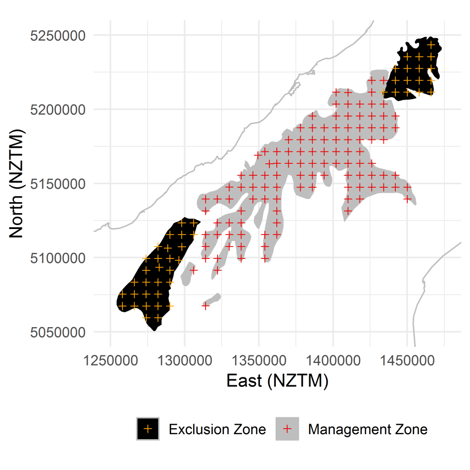Figure 1. Tier 1 locations where a vegetation plot has been sampled denoted according to the
exclusion and management zones.

A total of 126 and 34 Tier 1 sample locations correspond with the tahr management and
exclusion zones, respectively (Figure 1). Of these, 59 and 32 locations in the tahr
management and exclusion areas, respectively, have had at least one vegetation relevé
(“recce plot”) measurement; the remaining sample locations are either unvegetated (e.g.
permanent snow or ice) or have not yet had plots established. Of those locations where
relevés have been measured, 27 and 8 locations in the tahr management and exclusion areas,
respectively, have had additional vegetation measurements to assess tahr browse impacts
and quantify faecal pellets of ungulates. On 9 of these 35 plots, measurements of individual
tussocks had been made from between 4 and 6 subplots. Of these, 2 were in the exclusion
zone. We used all available vegetation and pellet data in this report.
3.2 Subjectively located plots
There are 117 subjectively located plots that sample 8 catchments within the tahr
management zone (Hooker-Tasman, Carney’s Creek (Rangitata), North Branch Godley, Arbor
Rift (Landsborough), Whymper (Whataroa), Fitzgerald (Godley), Townsend (Landsborough),
Zora (Landsborough); Cruz et al. 2017). Plot locations were intersected with the
management/exclusion zone layer (Figure 2).
- 4 -

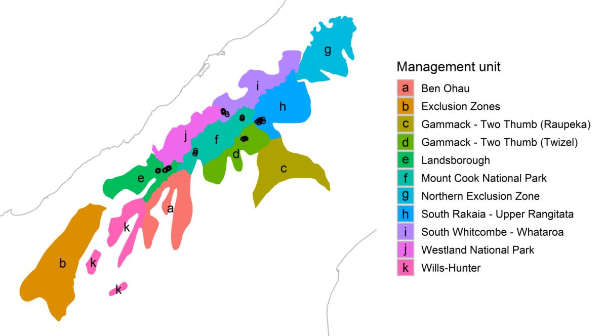Figure 2. Layout of the subjectively located plots with regard to the management units. In this
figure, each separate management unit as defined in the Himalayan Tahr Control Plan is shown.
The exclusion zones are named “Northern Exclusion Zone” and “Exclusion Zones”. These names
are as provided by the Department of Conservation. The black dots represent the subjectively
located plots.
3.3  Environmental covariates
Elevation, slope, aspect and geographical coordinates were obtained from direct field
measurements for all plots sampled for vegetation composition to date. We combined slope,
aspect and latitude to compute potential solar radiation (Kaufmann and Weatherred 1982), a
topographical direct solar irradiance index that accounts for northness where terrain is not
level.
Climate data were obtained for the Tier 1 plots and the subjectively located plots that occur
within the tahr management and exclusion areas. In the case of Tier 1 plots, the set of
planned but as yet unmeasured plots was also included in the assessment since plots will be
established at these sample locations in future. Climate data originate from NIWA’s spatial
layers. These data are median values from time series data, predicted from elevation, at a
resolution of 500 m × 500 m. Environmental variables considered were (1) mean annual
temperature (2) growing degree days (5°C base) (3) mean annual rainfall (4) soil moisture
deficit days (5) mean 9AM relative humidity (6) mean solar radiation (7) sunshine hours (50th
percentile) and (8) potential evapotranspiration (PET, with which we computed a Rainfall to
PET ratio).
Two sets of variables were found to be mutually collinear (|r | ≥ 0.80) or strongly correlated
across all sample locations (Table A1, Appendix 1). These were (i) elevation and the two
temperature variables and (ii) four moisture-related variables (rainfall, rainfall to PET ratio, soil
moisture deficit days and 50th percentile of sunshine hours). Two other variables, solar
radiation and relative humidity, were also correlated with this second set of variables but
- 5 -

link to page 17
more weakly so (0.33 ≤ |r | ≤ 0.72). All variables are presented but interpreted cautiously with
these correlations in mind.
3.4  Co-occurring animals
3.4.1  Identifying the likely presence of other introduced mammals in the
tahr management zone and tahr exclusion zone
We intersected the locations of the subjectively located plots and the Tier 1 vegetation plots
with the pest distribution polygons supplied by DOC (geodatabase
‘TahrMonitoringLCR_data.gdb’; all pest layers – e.g. ‘FallowDeer_2007’ and ‘FeralGoat_2014’,
hereafter “pest polygons”). This allowed us to consider for each zone type (exclusion or
management), the proportion of plots that fell within the mapped distribution of each pest.
Subsequently, we were provided with shapefiles for the distribution of tahr and chamois.
Unlike the shapefiles provided in TahrMonitoringLCR_data.gdb, which were polygons of
presence only, the tahr and chamois files included presence, “presence (determined on the
basis of tahr killed during control operations)”, absences, and modelled absences. We
subsetted the polygons to include only presence (including that determined from control
operations) polygons; we then applied the same workflow as above to determine whether
Tier 1 and pellet data fell within the tahr and chamois presence polygons. Figure 3 provides
an example of the methods for intersecting pellet and deer data with the pest polygons,
using red deer as an example.
- 6 -

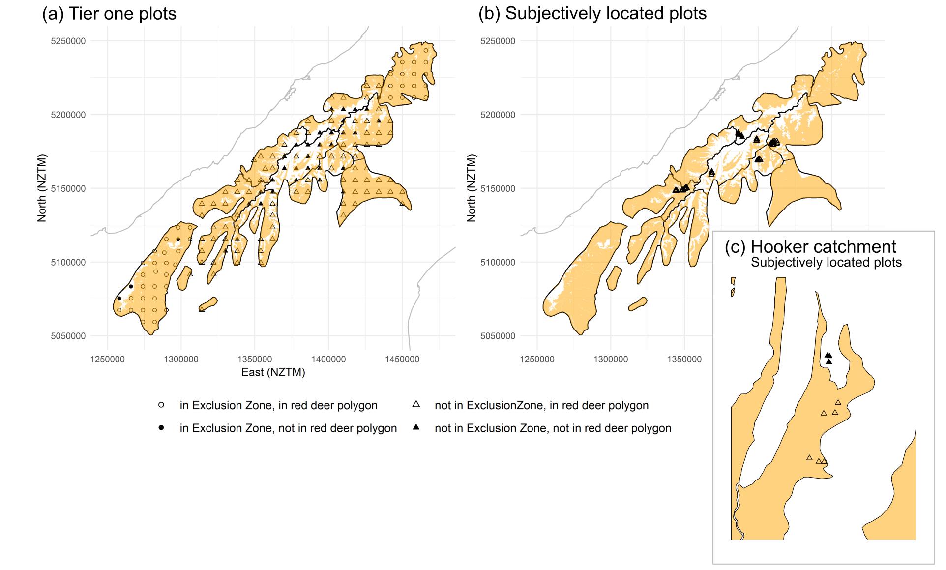Figure 3. Mapped distribution of red deer (orange polygons) within the tahr management area and the distribution of (a) Tier 1 plots and (b) and
subjectively located plots. (c) Shows a high-resolution version of the Hooker catchment (Mt Cook National Park management unit) of the subjectively
located plots.
- 7 -

3.4.2  Pellet data
Pellet counts were conducted between 2015 and 2017 at each Tier 1 sample location, at 5 m
intervals along each of four 150 m transects emanating diagonally from the corners of each
Tier 1 vegetation plot. At each 5-m interval, pellets were counted within circular plots of 1-m
radius for ungulate pellets and of 0.18-m radius for European rabbits (Oryctolagus cuniculus)
and hares (total 30 pellet plots per sample location). Ungulate pellets were counted
separately as intact and non-intact and were not differentiated to species, except for those
that were readily distinguished: cattle (Bos taurus), horse (Equus caballus), and pig (Sus
scrofa). Lagomorph pellets were not distinguished as intact or non-intact. Rabbits rarely
inhabit alpine tussock grasslands and, in these circumstances, lagomorph pellets are almost
always those of hares.
Pellets were counted along transects in the vicinity of the subjectively located plots (Cruz et
al. 2014, 2017), for all 8 catchments, between 2011 and 2013. The presence of pellets was
recorded on 1-m2 plots located on 8 × 20-m transects radiating from the central vegetation
plots and spaced at 5 m from each other (total 40 pellet plots per sample location). Ungulate
pellets can comprise those of tahr, chamois or red deer.
3.5  Vegetation communities
Vegetation data for both the Tier 1 plots and the subjectively located plots were extracted
from the National Vegetation Survey (NVS) databank. These data were used to assign plots to
pre-existing forest and shrubland alliances (Wiser et al. 2011, Wiser & De Cáceres 2013) or
non-woody alliances (Wiser et al. 2016) that had been defined in a national-scale, plot-based
classification (see section 4.31). To do this, it was critical to ensure that the names used for
plants on plots were consistent with those used to construct those alliances. First, we updated
all taxonomic names in the classifications, and in the vegetation plots to be assigned, to their
status according to Ngā Tipu o Aotearoa, the New Zealand Plants database
http://nzflora.landcareresearch.co.nz on 11 April 2018. Then, we deleted records of any taxa
not resolved at least to the genus level, following Peet and Roberts (2013). Owing to the
known inconsistencies of recording taxonomic levels below species, we aggregated all
subspecies and varieties to the species level. The most problematic situation was where there
were a mixture of genus-level and species-level identities in the same genus, on a plot (e.g.
two species of Chionochloa identified on a plot alongside Chionochloa sp.). For genera where
more than 30% of the records were at the genus level, we aggregated all species-level
records to the genus level. For genera where fewer than 30% of the records were at the
genus level, we deleted these lower-resolution records.
For all plots, two species importance value were constructed. The first was consistent with
that used in Wiser et al. (2011) and Wiser & De Cáceres (2013). For each species on each plot,
cover class midpoints were summed across tiers, with grassland tiers being consolidated to
match tiers used for woody vegetation (Hurst & Allen 2007). These were then converted back
to an ordinal value. The second was consistent with that used in Wiser et al. (2016). To ensure
comparability with earlier classification (Wiser et al. 2016), species were ranked from 1 = the
least abundant to n = the most abundant species on a plot (where n is equivalent to the total
- 8 -

number of species on the plot). Species with the same abundance measures on a plot were
assigned an equal, mean rank to derive an importance value for each.
For the ordination, we calculated a single importance value for each plant species as
described above for assignment to the woody classification. We also removed plant species
that only occurred once in the data – these species provide little information about major
compositional gradients because they cannot inform compositional distance between two
plots, being found on only one (Warton et al. 2015). The resulting ordination dataset had 208
plots and 452 vascular plant taxa (we removed 211 singletons). Of these 452 species, 443
occurred in the combined Tier 1 dataset (management and exclusion zone plots); only 9
species were found in the subjectively located plots that were not also found in the Tier 1
dataset. There were 224 species in the Tier 1 dataset that did not occur in the subjectively
located plots. This suggests the subjectively located plots sample a subset of the species pool
sampled by Tier 1 (as we would expect).
4
Methods
All statistical analyses were completed in R (R Core Team 2017).
4.1  Environmental covariate matching
The distribution and skewness of environmental variables was inspected before analysis.
Three variables with marked skewness (≥ 1) were log-transformed: rainfall to PET ratio,
sunshine hours and soil moisture deficit days. Variables were compared between the three
groups of plots (the Tier 1 management zone plots, the Tier 1 exclusion zone plots, and the
subjectively located plots) using linear models. We also compared soil pH and total
phosphorus from a subset of plots where soils had been collected and analysed for chemical
properties. Methods for soil chemical analyses follow Laughlin et al. (2015).
4.2  Co-occurring mammals
4.2.1  Pest animal distributions across the three plot groups
We calculated the proportion of plots that were within and outside of the mapped
distributions of each pest animal species, for the Tier 1 management zone plots, the Tier 1
Exclusion zone plots, and the subjectively located plots. The proportion of plots with/without
each pest animal species was compared across the three groups of plots using a generalised
linear model with binomial errors. Post hoc pairwise comparisons of mean proportions were
compared to the reference level of the subjectively located plots.
4.2.2  Pellets
We analysed the probability of observing faecal pellets across 30 to 40 pellet plots in each
sample location as an indication of ungulate and lagomorph activity (Cruz et al. 2014, 2017).
The analysis was based on generalized binomial models with count of pellet plots with and
- 9 -

without pellets in each sample location taken as response variable and plot groups (Tier 1
management zone plots, the Tier 1 Exclusion zone plots, and the subjectively located plots)
as a predictor. We controlled for different area of pellet plots between sample networks and
taxa by setting an offset for area of pellet plots and a conditional log-log link on the binomial
error structure (https://stats.stackexchange.com/questions/148699/modelling-a-binary-
outcome-when-census-interval-varies).
4.3  Vegetation communities
4.3.1  Classification
The development of the national-scale, plot-based vegetation classification, which formed
the basis of the analysis for this report, progressed through three main phases. The first
phase led to the creation of a (single-level) classification of national vegetation types based
on a relatively small, national-scale-plot data set sampled following a systematic design
(Wiser et al. 2011). This dataset was collected from 2002 to 2007, when 1177 20-m × 20-m
permanent vegetation plots were established at intersections of an 8-km × 8-km grid
superimposed on the areas mapped as shrubland or indigenous forest by the New Zealand
Land Cover Database (LCDB version 1; Thompson et al. 2004). Data were collected under the
auspices of the New Zealand Land Use and Carbon Analysis System (LUCAS; Coomes et al.
2002; Allen et al. 2003). The second phase developed a new classification approach, including
procedures to extend the initial classification system by incorporating 12,374 of pre-existing
vegetation plot records from the NVS databank (Wiser & De Cáceres 2013), to meet goals of
both allowing increased thematic resolution and allowing vegetation types that are rare on
the landscape to be defined. The third phase further extended the classification approach to
deal with inconsistencies in species abundance measurement protocols, a step that was
necessary to incorporate types describing non-forested vegetation into the classification
system (Wiser et al. 2016).
The classification extensions, that produced the final classifications for assignment used here,
used semi-supervised clustering with the fuzzy classification algorithm Noise Clustering (De
Cáceres et al. 2010). This approach allowed us to extend the pre-existing classifications while
retaining the previously described vegetation types and to identify vegetation plots that are
sufficiently distinct in their composition that they cannot be meaningfully grouped with other
plots to define a vegetation type, i.e. they are compositional outliers. This algorithm requires
two parameters: the fuzziness exponent (m) and the distance to the noise class (d). The
fuzziness exponent was set to m = 1.1 in all analyses. In the forest/shrubland classification the
distance to the noise class was d = 0.83. The value was chosen as the one that best matched
the initial classification of Wiser et al. (2011). This resulted in 29 vegetation types nationally at
the thematic resolution termed ‘alliances’ being defined. For the non-forested classification d
= 0.84. The slight differences in this parameter were necessitated by the use of relative ranks
as the abundance values creating a somewhat different resemblance space (Wiser et al.
2016). This resulted in 25 non-woody vegetation alliances being defined. All Noise Clustering
was centroid-based. Classifications at a final level of thematic resolution (termed
‘associations’) were also produced, but these are not used in the analysis presented in the
current report.
- 10 -

The analysis presented here used semi-supervised clustering with the fuzzy classification
algorithm Noise Clustering to assign each of the 208 vegetation plots (Tier 1 plots and the
subjectively located plots described in 3.5) to one of 29 forest or shrubland vegetation
alliances, to one of the 25 non-woody vegetation alliances. These assignments were done in
separate steps because of the difference in importance values and resemblance space in the
respective classifications. The parameters ‘m’ and ‘d’ took the values used in the respective
base classifications. All plots were assigned to the alliance (or the outlier class) to which they
had the highest fuzzy membership value, thus producing a ‘hard’ classification of these plots.
Further details are provided in Appendix 2.
The R packages vegan (Oksanen et al. 2011) and vegclust (De Cáceres et al. 2010) were used
for the classification and assignment analyses.
4.3.2 Ordination
We used non-metric multidimensional scaling (NMS), with Chord distance, to arrange plots in
multidimensional space based on their composition. NMS was implemented using metaMDS
in the vegan library of R (Oksanen et al. 2013; R Core Team 2017). Because of the high
compositional variability among plots (spanning forests, shrublands, grasslands and fellfield
vegetation types) we had 3128 plot pairs (14.5% of the total) that shared no species. This
high degree of species turnover among plots initially prevented the ordination reaching a
convergent solution so we implemented the step-across procedure to replace dissimilarities
with the shortest paths found by stepping across intermediate sites (Oksanen et al. 2013). We
established that three axes were needed to capture compositional variation (Appendix 3) and
reduce stress below 0.20. We then ran the NMS with 199 random starts and 4 repeat runs,
each one taking the best solution from the previous run. There are two methods for testing
differences in composition among groups of plots. One method uses a non-parametric
permutational approach to test for differences in the centroid (‘average’ composition) and
the spatial variability among samples (beta diversity, beta dispersion) (Anderson 2001), while
another method uses parametric generalised linear models to test for differences across
species (Wang et al. 2012). A key issue that led to the development of these two methods is
that while we are generally interested in differences in centroids, most contrasts of centroids
are confounded by differences among groups in the amount of dispersion (Warton et al.
2011). The parametric method claims to overcome this issue to provide a more confident test
of differences. As both methods have their merits and proponents, we apply both and report
and compare the results. For the non-parametric test, we used permutational multivariate
ANOVA (PERMANOVA) implemented with the function adonis in the vegan library of R, with
pairwise.adonis to test for differences between plot groups, and betadisper in the vegan
library of R to test for differences in beta dispersion among the three plot groups. For the
parametric method, we used the manyGLM function in the mvabund library of R (Wang et al.
2012).
In addition to formal statistical tests for differences among the three groups of plots, we
explored two ways of interpreting the ordination to gain ecological understanding of the
vegetation gradients. First, we interpreted the plot scores. In an NMS, each plot is assigned a
position along each of the three axes. We used 1-way ANOVA to test for differences in plot
scores along each axis among the three plots groups. We also used the envfit function in the
vegan library of R to fit vectors to each axis for elevation, MAR, MAT, percent ground cover,
- 11 -

link to page 36
bare ground and rock. Second, we interpreted the species scores. In an NMS, each species is
assigned a position along each of the three axes and we took these species scores and used
1-way ANOVA to test for differences in biostatus (native, non-native) to identify whether
communities at either end of each axis were characterised by non-native communities.
4.4  Palatable plant species used as indicators
Of the list of indicator species from McKay and McNutt (2016), we evaluated three tussock
grasses (Chionochloa spp.), seven spaniards (Aciphylla spp.) and three fleshy herbs (a
Celmisia and two Ranunculus species) (Table 4). All shrub species in plots are also measured
as indicators (McKay & McNutt 2016) but we do not consider them for this report since they
are likely to differ widely in their palatability to tahr and span a very wide range of
environments and life history strategies.
4.4.1  Frequency of each indicator species across the three plot groups
For the 12 non-shrub species, we first calculated the frequency of each species in each of the
three plot groups, and tested for statistical differences using generalised linear models with
binomial errors that account for the different number of plots in each plot group.
4.4.2  Climate space occupied by each indicator species
For the 12 non-shrub species, we downloaded all observations of each species from the
Global Biodiversity Information Facility (GBIF, www.gbif.org) that fell within the reported
geographic range of each species as reported in Mark (2014) and extracted mean annual
temperature (MAT) and mean annual rainfall (MAR) data for each location from the same
spatial layers described in Section 3.4 (completed by Richard Earl, DOC, June 2018). We
calculated the median, 5th, and 85th percentile values for MAT and MAR for each species and
compared these visually to the range of MAT and MAR sampled by each of the three plot
groups.
4.4.3  Tussock cover methods
For the tussock species, we compared two methods for measuring cover on plots. The first
method was visual estimates of percent cover (to the nearest 5%, or 1% for covers ≤4%) done
for each Chionochloa species listed in McKay & McNutt (2016) within each subplot. The
second method was measurements of individual tussock basal diameters, either done on all
individuals in a plot, or on individuals within a subsample of subplots (McKay & McNutt
2016). Estimates of total tussock cover were compared at the subplot-level and at the whole-
plot level using linear models.
4.4.4  Statistical power for tahr impact indicators
We determined the statistical power of the plot network to detect (i) a difference in
vegetation indicators between the two groups of Tier 1 plots (i.e. static differences from
point-in-time data), and (ii) differences in the rates of change of indicators between the plot
groups (i.e. temporal change). The sample size of the two groups of Tier 1 plots is fixed,
- 12 -

hence we focussed our assessment on the magnitude of differences or rates of changes that
the plot network could detect with sufficient (≥ 0.8) power, rather than determining the
number of plots necessary to detect a given effect size. Our choice of analysis technique
varied according to the statistical distribution of the response variable (Crawley 2007).
For point-in-time differences in basal area and crown cover of tussocks, we used the simR
package of Green et al. (2016). This approach estimates statistical power by simulation of
pilot study data (in this case the data from the Tier 1 plots).
For change in sum tussock cover, an arcsine transformation was sufficient for the data to
meet the assumptions of normality, so we used the power.t.test in R as a simple analytical
solution. Likely rates of change were estimated from the subjectively located plots that had
whole-plot tussock cover estimated in relevé cover classes at on two occasions. Once Tier 1
plots have been remeasured, these analyses could be repeated using data from Tier 1 plots.
For point-in-time differences in counts of Aciphylla spp. and Celmisia semicordata, and
percentage cover of Aciphylla spp., we used a simulation approach based on negative
binomial distributions and generalised linear models because the data were overdispersed
and not suitable for the simR package. Steps involved: (i) estimating the location and the
dispersion parameter for the negative binomial distribution with available data (by fitting
glm.nb in the MASS package with Tier 1 plot group as an explanatory variable and the
indicator data from the Tier 1 plots as response variables); (ii) running multiple simulations of
new data (with negative binomial distribution) of different sample sizes with pre-estimated
dispersion parameters and selected effect sizes; (iii) testing for differences in each simulated
dataset (with glm.nb); and (iv) computing statistical power as the proportion of datasets
where a significant effect was detected.
4.5  Propensity scoring models
We compared eight indicators of tahr impact between the Tier 1 plots in the exclusion zone
and in the management zone. The indicators were derived from the relevé (sum cover scores
across all species; sum cover scores for the Aciphylla species selected by McKay & McNutt
2016; sum cover scores for the Chionochloa species selected by McKay & McNutt 2016;
presence/absence of Ranunculus lyallii; presence/absence of one of the Chionochloa species
selected by McKay & McNutt 2016) or from the additional methods prescribed for Tier 1 tahr
plots (total shrub cover, estimated from the sum of individual covers; shrub cover where
shrubs were present, hence excluding the many zero values from the analysis; and mean
tussock height from the measurements of individual tussocks). The purpose of these
comparisons was to test whether there were differences in these indicators between the Tier
1 plots in the exclusion zone and the management zone.
Statistical comparisons were made using propensity scoring models. This analysis technique
uses environmental covariates for each plot to calculate the probability of a plot belonging to
one or other plot group, given the covariates. For comparability with previous analyses on
Tier 1 data, we followed the unpublished analysis provided by David Ramsay (Arthur Rylah
Institute, Australia) that was also based on Tier 1 data, and used the twang library in R to
estimate propensity scores for each plot. Propensity scores are computed according to
balancing rules that minimise covariate differences between treatment and control groups.
- 13 -

link to page 25 link to page 25 link to page 26 link to page 26
We applied mean effect size (“es.mean”) balancing, which minimise (i) the absolute
standardised bias (or effect size) for each covariate and (ii) the mean of the absolute
standardised bias across covariates. Diagnostic checks indicated that this method resulted in
satisfactory sample balancing (Appendix 4). Propensity scores were then used as weights in a
linear model (implemented in the survey library of R) to test for differences between the two
groups of plots. To aid interpretation, we also ran conventional GLM models comparing each
indicator between the two groups of Tier 1 plots to evaluate how propensity scoring affected
the results.
5
Results
5.1  Environmental covariate matching
The Tier 1 management zone plots had significantly higher elevations and hence colder mean
annual temperatures than the Tier 1 exclusion zone plots (temperature-related variables
(Figure 4). The subjectively located plots had significantly higher mean annual temperatures
than the Tier 1 management zone plots despite their elevations not being significantly lower
(Figure 4).
Most moisture-related variables and solar radiation (which generally tend to be correlated,
Table A1 in Appendix 1), are not significantly different between the Tier 1 management and
exclusion zone plots, with the exception of lower air humidity and lower sunshine hours in
the Tier 1 management zone (Figure 5). However, the subjectively located plots occurred on
sites that were wetter (higher rainfall, rainfall-PET ratios and lower periods of soil moisture
deficit) and with lower solar radiation, than the Tier 1 management zone plots (Figure 5).
Diagnostic checks indicated that the above results were robust to assumptions of
homogeneity of variance (Appendix 5).
Mineral soil pH data were available from 24 Tier 1 exclusion zone plots and 46 Tier 1
management plots. There was a highly significant difference in mineral soil pH between the
two groups of plots (linear model: F1,68 = 13.2, P = 0.00054) with a mean of 4.41 (± 0.14 1 SE)
in the exclusion zone and a mean of 5.04 (± 0.10 1 SE) in the management zone. Given that
pH is measured on a log-scale, this difference is ecologically meaningful and could reflect a
higher prevalence of raw soils in the management zone, relative to the exclusion zone.
However, total phosphorus (measured in 25 and 47 plots in the exclusion and management
zones, respectively) did not differ between the two zones (linear model: F 1,70 = 0.01, P =
0.924; mean for exclusion zone = 660.5 (± 45.3 1SE); mean for management zone = 655.2 (±
33.0 1SE). Total phosphorus is typically higher in raw soils so the lack of any difference in this
variable cf. the difference in pH warrants further investigation.
- 14 -

p
0.013
p  <0.001
a
b
ab
b
a
b
1400
) 7.0
C°( .
) 1300
p 6.5
m
m
(
et
e
l
d
a
u
6.0
t 1200
u
it
n
l
n
A
a n 5.5
1100
a
e
M 5.0
T1 Excl.
T1 Mgmt.
Subj. Mgmt.
T1 Excl.
T1 Mgmt.
Subj. Mgmt.
Sample

Sample

p
0.003
p
0.232
b
a
b
a
a
a
ys
a 900
d
32
e
)
er 800
°(
g

e
e 30
d
p
  700
o
g
l
n
S
i
w
28
600
or
G 500
26
T1 Excl.
T1 Mgmt.
Subj. Mgmt.
T1 Excl.
T1 Mgmt.
Subj. Mgmt.
Sample

Sample

p
0.321

a
a
a
n 0.80
oitaidar  0.75
r
al
so .to 0.70
P
T1 Excl.
T1 Mgmt.
Subj. Mgmt.
Sample

Figure 4. Environmental contrast between tahr exclusion and management areas corresponding
to Tier 1 or subjectively located plots. The statistical significance of the linear model as P values
and error bars illustrate confidence intervals. Different letters on top of boxes indicate that
treatment levels were significantly different from each other (Tukey test, P > 0.05).
- 15 -

p  <0.001
p
0.013
a
a
b
a
a
b
)
m
20
m(
o
  7000
i
l
t
l
a
a
r
f
  15
n
T
i
a 6000
E
r
P
l

a
ot
u
l 10
n 5000
l
n
af
a
ni
n
a
a 4000
R
e
M 3000
5
T1 Excl.
T1 Mgmt.
Subj. Mgmt.
T1 Excl.
T1 Mgmt.
Subj. Mgmt.
Sample
Sample

p  <0.001
p  <0.001
c
b
a
ab
b
a
25
1600
ys
a
s
d
r
t 20
u
ci
o 1500
if
h
e 15
e
d
ni
e
1400
r
u
sh
n
sti
u
o 10
S 1300
m lioS
T1 Excl.
T1 Mgmt.
Subj. Mgmt.
T1 Excl.
T1 Mgmt.
Subj. Mgmt.
Sample
Sample

p  <0.001
p
0.037
)
b
b
a
b
a
ab
2
12.9
)
m
% 82.5
(
J
y
M
t
(
i

12.8
d 82.0
n
i
oi
m
t
u 81.5
ai 12.7
h
d
ar
ve

it 81.0
r
a
a
12.6
l
l
er 80.5
so

n
n
12.5
a
a
e
e
80.0
M
M
T1 Excl.
T1 Mgmt.
Subj. Mgmt.
T1 Excl.
T1 Mgmt.
Subj. Mgmt.
Sample
Sample

Figure 5. Environmental contrast between tahr exclusion and management areas corresponding
to Tier 1 or subjectively located plots. The statistical significance of the linear model as P values
and error bars illustrate confidence intervals. Different letters on top of boxes indicate that
treatment levels were significantly different from each other (Tukey test, P > 0.05).

- 16 -

link to page 27 link to page 27 link to page 27

5.2  Co-occurring mammals
5.2.1  Identifying the likely presence of other introduced mammals in the
tahr management zone and tahr exclusion zone
The primary concern was whether there were differences in the co-occurrence of other
herbivores with tahr in this environment. The critical comparisons in Figure 6 are between the
subjectively located plots and the Tier 1 management zone plots (because impacts might be
compared between these two plot groups where tahr occur) and between the Tier 1
management zone plots and the Tier 1 exclusion zone plots (because these are used as a
‘treatment’ and ‘control’ to assess impacts).
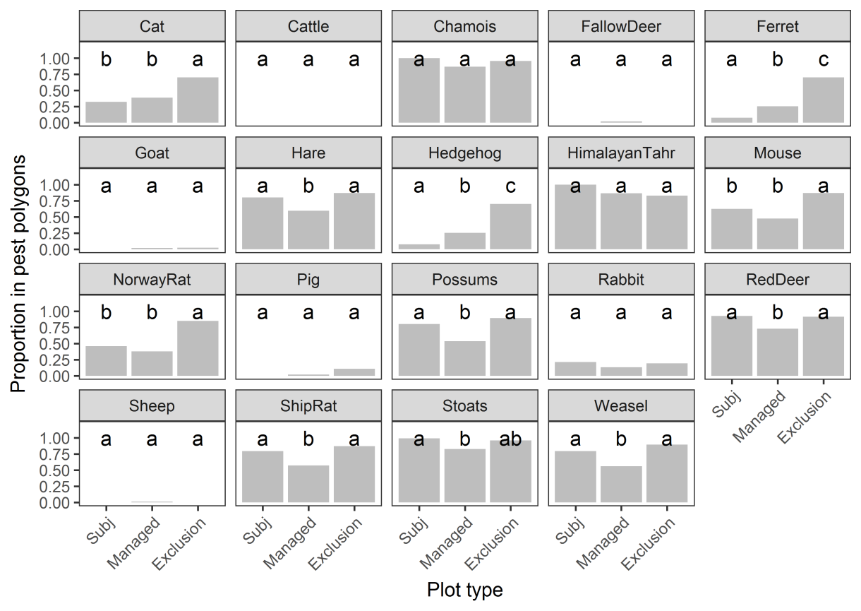
Eight pest species differed in their distribution between the subjectively located plots and the
Tier 1 management zone plots (ferret, hare, hedgehog, possum, red deer, ship rat, stoat,
weasel; Figure 6). This means that when comparing vegetation indicators between these two
plot groups, differences may be attributable to tahr, but could also reflect differences in the
presence or abundance of any of those eight species (particularly the herbivores and
omnivores).
Ten pest species differed in their distribution between the Tier 1 management zone plots and
the Tier 1 exclusion zone plots (cat, ferret, hare, hedgehog, mouse, Norway rat, possum, red
deer, ship rat, weasel; Figure 6).

Figure 6. Proportion of plots within mapped polygons of pest species (raw mean). Bars with
different letters are statistically different at P < 0.05. ‘Subj’ = subjectively located plots;
‘Managed’ = Tier 1 plots in the management zone; ‘Exclusion’ = Tier 1 plots in the exclusion
zone.
- 17 -

link to page 28 link to page 28 link to page 28 link to page 28 link to page 28 link to page 27

5.2.2  Pellets
Intact ungulate pellets occurred more frequently in the Tier 1 management zone plots than in
the Tier 1 exclusion zone plots (Figure 7a). Ungulate pellets were nearly 8 times more
frequent in subjectively located plots than in the Tier 1 management zone plots (Figure 7a).
The frequency of ungulate pellets was higher when non-intact pellets were also accounted
for (Figure 7c) relative to when only intact pellets were taken into account (Figure 7a) but the
general pattern remained unchanged. The frequency of hare pellets was very similar between
Tier 1 management zone plots and Tier 1 exclusion zone plots but these were both
significantly higher than their frequency in subjectively located plots (Figure 7b). These results
contrast markedly with the differences reported above from the mapped distribution of hares
(Figure 6) and underscore the value of plot-specific measurements of animal abundance as a
strength of the Tier 1 monitoring approach.
a)
b)
p  <0.001
p  <0.001
)
2
)

0.30

2
0.55
(m
0.25
s
m
t
0.20
( 0.50
ell 0.15
s t
e
el
p
l
0.45

0.10
e
et
p
al
e
0.40
u
r
0.05
g
a
n
h f 0.35
u f
o .
o .
b
0.30
b
or
or
P
P
T1 Excl.
T1 Mgmt.
Subj. Mgmt.
T1 Excl.
T1 Mgmt.
Subj. Mgmt.
Sample
Sample

c)

p  <0.001
)
2

0.30
(m 0.25
s t 0.20
elle 0.15
p et 0.10
alugn 0.05
u fo .borP
T1 Excl.
T1 Mgmt.
Subj. Mgmt.
Sample

Figure 7. Probabilities of observing ungulate or hare pellets within 1-m2 tahr management and
exclusion areas with objectively (Tier1) or subjectively (Subj.) located sampling networks.
Estimates for ungulate pellets are presented for (a) intact and (c) for combined intact and non-
intact pellets.
- 18 -

5.3  Vegetation communities
5.3.1  Classification
Of the plots that were aligned to pre-defined communities, 65% of those in the subjectively
located plots were non-woody, compared with just 24% in the Tier 1 management zone, and
just 19% in the Tier 1 exclusion zone (Table 1). In contrast, of the plots that were aligned,
more than one third (38%) of the plots in the Tier 1 exclusion zone were woody, compared
with just 15% in the Tier 1 management zone and < 1% in the subjectively located plots
(Table 1). Importantly, at least one third of the plots in each group were assigned to the
outlier class (Table 1), which limits the scope for comparing alliances across the three plots
groups.
Plots that could be assigned to non-woody classes were variously distributed across ten
different alliances, dominated by various Chionochloa species and native short tussocks. That
over half of the assigned subjectively located plots were assigned to type T3 (Chionochloa
pallens / Poa colensoi–Chionochloa crassiuscula–Celmisia lyallii tussockland), in comparison
with only one of the Tier 1 plots (in the management zone), and that no subjectively located
plots were assigned to type T6 (Chionochloa macra–Poa colensoi / Celmisia lyallii–[Luzula
rufa] tussockland), in comparison to four Tier 1 plots (also in the management zone),
demonstrates the compositional bias in the dataset of subjectively located plots.
Most of the plots assigned to a woody vegetation alliance were sampled by one of the two
Tier 1 plot groups, not by the subjectively located plots. These were variously distributed
across nine different woody alliances, including montane and subalpine shrublands, beech
forest, and forests dominated by kāmahi (Weinmannia racemosa) (Table 1).
In addition to this classification, we made a simple classification of all plots on the basis of
whether half or more of the sum cover was from woody species. This allowed us to partition
the outlier plots into ‘woody’ or ‘non-woody’. From this, we estimate that 87% of the
subjectively located plots are non-woody (102 out of 117), 73% of the Tier 1 management
zone plots are non-woody (43 out of 59 plots), and 47% of the Tier 1 exclusion plots are non-
woody (15 out of 32 plots).
- 19 -

Table 1. Summary of plot assignations to the woody (Wiser et al. 2011; Wiser & De Cáceres 2013) and non-woody (Wiser et al. 2016) national plot-based
classifications. ‘Subj’ = subjectively located plots; T1 Excl = Tier 1 plots in the exclusion zone; T1 Mngt = Tier 1 plots in the management zone. The number
(percentage in brackets) of plots in each of these groups that are either in woody vegetation, non-woody vegetation or designated as an outlier is
provided
Physiognomic
Code
Community
Subj
T1
T1
Group
Mngt
Excl
Tussockland
T1
Chionochloa crassiuscula–Schoenus pauciflorus–Poa colensoi / Astelia linearis tussockland
14
1
1
Tussockland
T2
Chionochloa pallens / Poa colensoi / Anisotome aromatica–Gaultheria depressa tussockland
1
0
0
Tussockland
T3
Chionochloa pallens / Poa colensoi–Chionochloa crassiuscula–Celmisia lyallii tussockland
39
1
0
Tussockland
T4
[Chionochloa pallens] / Poa colensoi–Celmisia petriei–Schoenus pauciflorus / Wahlenbergia albomarginata tussockland
12
1
2
Tussockland
T5
Chionochloa rigida / Poa colensoi–Festuca novae-zelandiae / Hypochaeris radicata tussockland
6
2
0
Tussockland
T6
Chionochloa macra–Poa colensoi / Celmisia lyallii–[Luzula rufa] tussockland
0
4
1
Tussockland
T8
Festuca novae-zelandiae–Poa colensoi–Anthoxanthum odoratum / Leucopogon fraseri tussockland
1
1
0
Tussockland
T9
Festuca novae-zelandiae / Anthoxanthum odoratum–Trifolium repens–Hypochaeris radicata grassland
0
1
0
Tussockland
T10
Poa colensoi–Rytidosperma setifolium–Festuca matthewsii / Wahlenbergia albomarginata tussockland
1
1
1
Grassland
G6
Poa colensoi / Chionochloa oreophila, Celmisia sessiliflora, Celmisia haastii grassland
2
2
1
Shrubland
A: S4
Discaria toumatou – Coprosma propinqua / Anthoxanthum odoratum – Dactylis glomerata shrubland
0
0
1
Shrubland
A: S5
Dracophyllum uniflorum / Gaultheria crassa – Poa colensoi – Festuca novae-zelandiae montane shrubland
1
0
0
Shrubland/Forest
A: PF1
Dracophyllum traversii – Dracophyllum longifolium – Coprosma pseudocuneata – Archeria traversii low forest and
0
0
1
subalpine shrubland
Forest
A: BBLF1
Weinmannia racemosa – Griselinia littoralis – Pseudowintera colorata / Blechnum discolor forest
0
3
0
Forest
A: BBLF2
Nothofagus menziesii – Griselinia littoralis – Myrsine divaricata / Coprosma foetidissima forest
0
2
5
Forest
A: BBLF3
Nothofagus menziesii – Weinmannia racemosa – Nothofagus fusca / Blechnum discolor forest
0
0
1
Forest
A: BF3
Nothofagus solandri – (Nothofagus fusca) / Coprosma microcarpa – Leucopogon fasciculatus forest
0
0
1
Forest
A: BF5
Nothofagus menziesii / Hoheria glabrata – Myrsine divaricata – Coprosma ciliata / Polystichum vestitum montane forest
0
3
3
Forest
A: BLPF1
Weinmannia racemosa – Prumnopitys ferruginea – Dacrydium cupressinum / Blechnum discolor forest
0
1
0
- 20 -

Physiognomic
Code
Community
Subj
T1
T1
Group
Mngt
Excl
Non-woody

76
14
6
(65%)  (24%)  (19%)
Woody

1
9
12
(<1%)  (15%)  (38%)
Outlier

40
36
14
(34%)  (61%)  (44%)

TOTAL
117
59
32
- 21 -

5.3.2 Ordination
A three-axis NMS ordination reached a satisfactory convergent solution with a stress of 0.159
and non-metric goodness of fit between ordination distances and original dissimilarities of
0.95 (Appendix 3). Beta dispersion differed among the three plot groups (F2,205 = 41.1, P <
0.001) with pairwise differences between the subjectively located plots and either Tier 1 plot
group (both P < 0.001), but not between the two Tier 1 plot groups (P = 0.070) (Figure 8).
These patterns were driven by the comparatively low beta dispersion among the subjectively
located plots. Both the non-parametric and parametric tests pointed to a difference in
composition among the three groups, but given the large differences in dispersion among
plot groups, these results should be interpreted cautiously (PERMANOVA F2,205 = 7.88, P =
0.001; all pairwise differences P < 0.05, strongest between each Tier 1 group and the
subjective plots (P = 0.003) and least between the two Tier 1 plot groups P = 0.012;
manyGLM: test statistic = 36.4, P < 0.001, all pairwise differences P < 0.001) (Figure 8).
Plot scores along Axis 1 were sorted by elevation, mean annual temperature (MAT) and, more
weakly so, percent rock cover and percent ground cover (Table 2). Low axis 1 scores were
associated with high elevation, rocky ground, and scree species, while high axis 1 scores were
associated with low elevation and forest species (Table 3). Each plot group differed from each
other plot group on axis 1 scores (ANOVA, F2, 205 = 23.6, P < 0.001) (Figure 8). The Tier 1
exclusion zone plots had higher axis 1 scores than the other two plot groups reinforcing that
this plot group includes low elevation, forested vegetation. Species scores along axis 1 did
not differ between native and non-native species (ANOVA, F1, 432 = 0.60, P = 0.44).
Plot and species scores along Axis 2 were sorted by percent rock and ground cover and,
more weakly so, elevation, MAT and MAR (Table 2). Low axis 2 scores were associated with
open ground at high elevation, while high axis 2 scores were associated with lower elevation
sites and species that occur on sites with poor drainage (Table 3). Each plot group differed
from the other plot groups on axis 2 scores (ANOVA, F2, 205 = 37.6, P < 0.001), although the
difference between the Tier 1 plots in the tahr exclusion zone and the subjectively located
plots was only significant at P = 0.05) (Figure 8). The Tier 1 plots in the tahr management
zone had the lowest axis 2 scores, and the subjectively located plots had the highest scores
suggesting a difference in elevation and drainage between these two groups. Species scores
along axis 2 differed significantly between native and non-native species (ANOVA F1, 432 =
8.14, P = 0.005) – non-native species had lower axis 2 scores corresponding to open ground
and cooler climates.
Axis 3 plot scores did not differ among the three plot groups (ANOVA F2, 205 = 0.82, P = 0.44)
(Figure 8). Axis 3 was the hardest to interpret but the clearest relationship was with mean
annual rainfall (Table 2). Higher axis 3 scores were drier than lower axis 3 scores and those
drier plots hosted species typically found east of the Main Divide (e.g. Discaria toumatou)
(Table 3). Species scores along axis 3 differed significantly between native and non-native
species (ANOVA F1, 432 = 42.1, P < 0.001) – non-native species had higher axis 3 scores, again
corresponding to drier locations, east of the Main Divide (e.g. High Country lands).
- 22 -

2
3
1
S
S
S
M
M
M
N
N
N
Subj
T1Excl
T1Mng
NMS 1
NMS 2
NMS 3
5.
0
1
.
5.
1
0
0
.
1
5
5
0
.
.
.
1
0

0
2
0

3
si
si
si
x
x
x
a
a
5

.
a
0
S
0
S
-
.
S
0
5
M
.
M
M
N
0-
N
0
N
.
1-
5.0-
5
5
.
.
1
1
-
-
0.1-
Subj
T1Excl
T1Manage
Subj
T1Excl
T1Manage
Subj
T1Excl
T1Manage
2.0
1.5
1.5
0.5
1.0
1.0
1
0.0

2
3
si
si
si
x
0.5
0.5
x
x
a
a -0.5
a
S
S
S
M
0.0
M
M
N
N
0.0
N
-1.0
-0.5
-0.5
-1.5
-1.0
br
di
b
nr
e
nr
di
br
nr
nr
b
e
nr
br
nr
di
e
b
o
o
ur
e
er
e
o
o
e
e
ur
er
e
o
e
o
er
ur
F
ni
h
F
T
f
f
f
e
ni
F
F
e
h
T
e
F
F
ni
T
h
m
S
e
m
e
S
e
m
S
a
r
r
r
r
T
ar
T
T
ar
G
G
G

Figure 8. Three biplots capturing the three non-metric multidimensional scaling axes. First row shows each plot group in bivariate space (3 biplots are
required for a 3-axis NMS). The second row shows the axis 1, 2 and 3 plot scores by plot group. ‘Subj’ = subjectively located plots; ‘T1Ex’ or ‘T1 Excl’ = Tier
1 plots in the exclusion zone; ‘T1Mng’ or ‘T1 Manage’ = Tier 1 plots in the management zone.
- 23 -

Table 2. Environmental vectors for each non-metric multidimensional scaling (NMS) axis,
determined using envfit. NS = relationship non-significant (P > 0.05). Otherwise, we show the r2
with the direction of the relationship in parentheses and statistical significance as follows: *** =
P < 0.001; ** = P < 0.01; * = P < 0.05
Plot-level variable
NMS 1
NMS 2
NMS 3
Elevation
0.49 (-ve) ***
0.04 (-ve) **
NS
Rock
0.08 (-ve) ***
0.45 (-ve) **
NS
Ground cover
0.03 (+ve) *
0.33 (+ve) ***
NS
MAT
0.25 (+ve) ***
0.05 (+ve) **
NS
MAR
NS
0.03 (+ve) **
0.45 (-ve) ***
Bare ground
NS
NS
NS
Physiography†
NS
NS
NS
† Physiography was a categorical variable with four values (gully, terrace, face, ridge) and a centroid was fitted for
each value. All other variables were continuous and numeric.

Table 3. Species with high and low non-metric multidimensional scaling (NMS) axis scores. First
10 species on each axis. * = non-native

NMS 1
NMS 2
NMS 3
Low (-ve)
High elevation scree and rock
High elevation open ground
Mostly low-stature species of
values

fellfield, etc.

Agrostis magellanica
Colobanthus buchananii
Anisotome imbricata
Colobanthus acicularis
Colobanthus canaliculatus
Anisotome pilifera
Colobanthus monticola
Colobanthus monticola
Carex pyrenaica
Epilobium pycnostachyum
Epilobium crassum
Colobanthus canaliculatus
Kelleria croizatii
Epilobium porphyrium
Colobanthus monticola
Kelleria villosa
Epilobium tasmanicum
Dracophyllum pubescens
Ranunculus sericophyllus
Haastia sinclairii
Luzula colensoi
Raoulia buchanani
Lachnagrostis filiformis
Poa hesperia
Raoulia eximia
Ourisia sessilifolia
Raoulia tenuicaulis
Veronica ciliolata
Poa novae-zelandiae
Veronica ciliolata
High (+ve)  Low elevation forest
Lower elevation, ground cover,  East of the divide
values

wet

Blechnum discolor
Anemone tenuicaulis
Acrothamnus colensoi
Carex imbecilla
Carex geminata
Chionochloa rigida
Dicksonia squarrosa
Celmisia armstrongii
Colobanthus acicularis
Earina autumnalis
Coprosma crenulata
Dianthus species*
Metrosideros diffusa
Drosera stenopetala
Discaria toumatou
Microlaena avenacea
Hierochloe novae-zelandiae
Festuca novae-zelandiae
Muehlenbeckia australis
Leptecophylla juniperina
Geranium brevicaule
Prumnopitys ferruginea
Oreobolus pectinatus
Geranium sessiliflorum
Pyrrosia eleagnifolia
Veronica macrantha
Hypericum perforatum*
Schefflera digitata
Veronica odora
Scleranthus uniflorus
- 24 -

link to page 36 link to page 36 link to page 36 link to page 36
5.4  Palatable plant species used as indicators
The merits and limitations of the indicators and methods used to derive indicators are
covered in the Discussion (Section 6.6). In this section, we summarise the frequency of each
indicator species across the three plot groups, summarise the climate space where each
indicator species occurs relative to the climate space in each of the three plot groups, and
assess whether the individual-level measurements of tussocks yield a similar estimate of total
cover to the subplot-level and whole-plot level estimates of cover.
5.4.1  Frequency of each indicator species across the three plot groups
The frequencies of all indicator species were statistically similar between the two Tier 1 plot
groups (Table 4). The only statistical differences were between the two Tier 1 plot groups and
the subjectively located plots (Table 4) and the species that differed were Chionochloa
pallens, Chionochloa flavescens and Aciphylla divisa. The herb Aciphylla horrida was absent
from the subjectively located plots and found in <10% each of the two Tier 1 plot groups
(Table 4), and Aciphylla colensoi was only sampled once, from a Tier 1 plot in the
management zone (Table 4). Ranunculus godleyanus was not sampled in any of the plots (as
anticipated by McKay & McNutt 2016).
These data suggest that inferences drawn from the subjectively located plots might not be
equivalent to those drawn from the Tier 1 plots. For example, an indicator based on tussocks
from the subjectively located plots will be largely informed by Chionochloa pallens, while the
same indicator from the Tier 1 exclusion plots will be informed more by Chionochloa
flavescens. If the ecology of these two species is different (see Section 6. Discussion), a
pooled indicator might conflate grazing processes with other processes driving the
distribution and abundance of the species. However, if the ecology of the two species is
comparable, or the grazing effect size is very large relative to the effect sizes from other
processes, this might not be an issue.

- 25 -

link to page 38 link to page 37
Table 4. Frequency of indicator species (expressed as proportions) in each group of plots.
χ2 and P values are from a GLM (df = 2) testing for differences in frequency of each species
across plot groups. Post-hoc differences are P < 0.05. NA = too few occurrences to model across
plot groups
Indicator
Indicator species
Subjective (N
Tier 1
Tier 1
GLM χ2
group
= 117)
Management
Exclusion   (P)
(N = 59)
(N = 32)
Tussocks
Chionochloa pallens
0.82 a
0.29 b
0.47 b
52.0 (< 0.001)
Chionochloa flavescens
0.15 a
0.17 ab
0.34 b
5.82 (0.054)
Chionochloa rigida
0.15
0.19
0.19
0.64 (0.726)
Spaniards
Aciphylla aurea
0.17
0.17
0.19
0.06 (0.973)
Aciphylla divisa
0.21 a
0.05 b
0.13 ab
9.37 (0.009)
Aciphylla crenulata
0.18
0.10
0.13
2.12 (0.347)
Aciphylla montana
0.02
0.03
0.03
0.55 (0.760)
Aciphylla scott-thomsonii
0.02
0.02
0.03
0.25 (0.881)
Aciphylla horrida
0
0.07
0.09
NA
Aciphylla colensoi
0
0.02
0
NA
Fleshy herbs  Celmisia semicordata
0.21
0.17
0.34
3.63 (0.163)
Ranunculus lyallii
0.30
0.22
0.28
1.27 (0.531)
Ranunculus godleyanus
0
0
0
NA

5.4.2  Climate space occupied by each indicator species
Aggregating across palatable species can be a statistically powerful approach for reporting
on ungulate impacts across plot networks. The key advantage is the gain in statistical power
from drawing on many species with a similar functional response to grazing, rather than
relying on individual species that have may limited distributions across the plot network. The
approach relies on the individual species having similar functional responses to grazing, and
broadly similar ecological attributes such that any aggregated response can be confidently
attributed to grazing rather than other factors. The approach could be further confounded by
the responses of individual species if there are few plots and few palatable species, and if the
palatable species are sorted along environmental gradients that are not equally represented
in the plots of each treatment group.
We summarised the climate across locations where each indicator species has been recorded
in GBIF. From this simple analysis, we observed that the 12 indicator species split into 3
groups – low, medium and high rainfall species (Figure 9; Table 5). This is just one dimension
of the ecology of each species that could be taken into account when aggregating across
species. One possibility to consider is to group the indicator species by rainfall until such time
as their biology and palatability is understood in more detail. However, we emphasise that
without detailed ecological information on each species (see Section 8, Recommendations,
below), there is a risk that aggregating across species with widely differing environmental
niches, will undercut the power of the ecological indicator to detect change related to
grazing.
- 26 -

Table 5. Summary statistics of mean annual rainfall (MAR) and mean annual temperature (MAT)
for each of the 12 indicator species. Data are the (5th)-median -(95th) percentiles for MAR and
MAT for each species based on all records in GBIF that fall within the reported geographic range
in Mark (2014). Species are grouped according to median MAR (< 2000 mm; 2000–4000 mm;
>4000 mm). Herbivores known to select these species are indicated (‘known drivers’)
Species
Known drivers
MAR (mm)
MAT (°C)
Aciphylla aurea
Fire, Hares1, Sheep2
(551) - 1151 - (3236)
(5.0) - 7.3 - (9.9)
Aciphylla scott-thomsonii
Pigs3
(603) - 1262 - (5814)
(5.0) - 7.4 - (11.6)
Chionochloa rigida
Tahr4,5, chamois6, hare6
(606) - 1356 - (5553)
(4.5) - 6.7 - (9.8)
Aciphylla montana
Tahr6
(597) - 1512 - (7651)
(3.2) - 5.5 - (7.7)
Aciphylla colensoi

(1411) - 2922 - (8551)
(4.9) - 7.2 - (10.0)
Chionochloa flavescens
Tahr4,5, chamois6, hare6
(1278) - 3030 - (8721)
(4.4) - 6.7 - (10.4)
Celmisia semicordata

(1025) - 3283 - (10004)
(4.1) - 6.6 - (12.8)
Chionochloa pallens
Tahr4,5, chamois6, hare6,7
(1504 - 3373 - (9500)
(4.0) - 6.2 - (9.5)
Aciphylla divisa

(1456) - 4196 - (9566)
(3.0) - 5.6 - (7.5)
Aciphylla horrida
Tahr8
(653) - 4440 - (9351)
(4.1) - 6.8 - (8.2)
Ranunculus lyallii
Snowbanks & flushes
(2325) - 4919 - (10004)
(3.8) - 6.3 - (8.3)
Tahr9, chamois6,
Aciphylla crenulata

(1675) - 5117 - (9772)
(3.6) - 6.1 - (8.7)
1Campbell (1981); 2Norton & Young (2016); 3 Walker et al. (2001); 4 Rose & Allen (1990); 5 Thomson et al. (1997); 6
Parkes & Thomson (1995); 7 Flux (1967); 8 Wardle (1979); 9 Tustin & Parkes (1988)
- 27 -

Aciphylla aurea
Chionochloa rigida
Aciphylla scott-thomsonii
Aciphylla montana
13000
13000
13000
13000
)
)
)
)
m
m
m
m
m(
m
m
m

(
(
(
ll

5000
ll
5000
ll
5000
ll
5000
af
af
af
af
ni
n
n
n
3000
i
i
i
a
3000
a
3000
a
3000
a
R
R
R
R
l

2000
l
l
l
a
2000
a
2000
a
2000
a
u
u
u
u
n
n
n
n
n
n
n
n
A
1000

A
1000

A
1000

A
1000

n
n
n
n
a
a
a
a
e
e
e
e
500
M
500
M
500
M
500
M
300
300
300
300
0
2
4
6
8
10
12
14
0
2
4
6
8
10
12
14
0
2
4
6
8
10
12
14
0
2
4
6
8
10
12
14
Mean Annual Temperature ( C)
Mean Annual Temperature ( C)
Mean Annual Temperature ( C)
Mean Annual Temperature ( C)
Chionochloa flavescens
Aciphylla colensoi
Celmisia semicordata
Chionochloa pallens
13000
13000
13000
13000
)
)
)
)
m
m
m
m
m(
m
m
m

(
(
(
ll

5000
ll
5000
ll
5000
ll
5000
af
af
af
af
ni
ni
ni
ni
a
3000
a
3000
a
3000
a
3000
R
R
R
R
l

2000
l
l
l
a
2000
a
2000
a
2000
a
u
u
u
u
n
n
n
n
n
n
n
n
A
1000

A
1000

A
1000

A
1000

n
n
n
n
a
a
a
a
e
e
e
e
500
M
500
M
500
M
500
M
300
300
300
300
0
2
4
6
8
10
12
14
0
2
4
6
8
10
12
14
0
2
4
6
8
10
12
14
0
2
4
6
8
10
12
14
Mean Annual Temperature ( C)
Mean Annual Temperature ( C)
Mean Annual Temperature ( C)
Mean Annual Temperature ( C)
Aciphylla horrida
Aciphylla divisa
Ranunculus lyallii
Aciphylla crenulata
13000
13000
13000
13000
)
)
)
)
m
m
m
m
m(
m
m
m

(
(
(
ll

5000
ll
5000
ll
5000
ll
5000
af
af
af
af
ni
n
n
n
3000
i
i
i
a
3000
a
3000
a
3000
a
R
R
R
R
l
2000
l
l
l
a
2000
a
2000
a
2000
a
u
u
u
u
n
n
n
n
n
n
n
n
A
1000

A
1000

A
1000

A
1000

n
n
n
n
a
a
a
a
e
e
e
e
500
Subjective
M
500
M
500
M
500
M
T1 Exclusion
300
300
300
300
T1 Management
0
2
4
6
8
10
12
14
0
2
4
6
8
10
12
14
0
2
4
6
8
10
12
14
0
2
4
6
8
10
12
14
Mean Annual Temperature ( C)
Mean Annual Temperature ( C)
Mean Annual Temperature ( C)
Mean Annual Temperature ( C)

Figure 9. Indicator species displayed in terms of climate space sampled by the three plot groups (shown as hulls) with the median climate of each indicator
species shown as an open symbol with the 5th and 9th percentiles of climate shown as bars. Species are organised from the top left to the bottom right, in
order of the median mean annual rainfall where they are found in New Zealand.
- 28 -

link to page 39 link to page 39 link to page 39 link to page 40 link to page 40

5.4.3 Tussock cover methods
The basal area of tussocks was positively related to visual estimates of crown cover at the
scale of both the subplot (Figure 10a) and plot (Figure 10b). The relationship was strong at
both scales, with visual estimates of crown cover (to the nearest 5%) predicting the more
accurate estimates of basal area (projected from direct measurements of individual basal
diameter) with good confidence, as shown by R2 values. The relationship illustrates the typical
crown spread of tillers relative to the base of tussock plants, with a slope of c. 0.23, well
below the 1:1 line (Figure 10a,b). It can also be noted that, at subplot level, prediction
intervals were wider at large cover values indicating that visual estimates of crown cover
could correspond to a wide range of basal area values (with 95% probability).
a) Subplots
b) Plots
35
2
1:1
R
0.72
)
)
60
2
30
1:1
2
2
m(
m
R
0.71

(
a
25
50
a
er
er
a
a
l

20
l
40
sa
sa
a
a
b
15
b
30

d
d
e
e
ct
10
ct
e
20
j
e
o
j
r
o
5
r
P
P
10
0
0
0
5
10
15
20
25
0
10
20
30
40
50
60
2

Estimated crown cover (m )

2

Estimated crown cover (m )

Figure 10. Basal area versus crown cover of tussocks (a) within 25-m2 (5 m × 5m) subplots and
(b) within whole 400-m2 (20 m × 20 m) plots from all Tier 1 plots across the tahr management
and exclusion zones. Each regression line is presented with confidence intervals (dashed line).
Prediction intervals based on a flexible spline estimate of mean squared error1 (dotted lines) are
also presented in (a). Double absences were excluded from the analysis.
5.4.4 Statistical power for tahr impact indicators
Point-in-time differences in tussock basal area and crown cover
The power analysis estimated that 30 Tier 1 plots (20 m × 20 m) in each of the tahr
management and exclusion zones are sufficient to detect a difference in tussock basal area of
ca. 6% (Figure 11a). Using the same number of plots, there is only sufficient statistical power
to detect a c. 20% difference in tussock cover between the zones (Figure 11b). The power
analyses express effect sizes as percentages, not absolute amounts. A 1 m2 increment of

1 https://stats.stackexchange.com/questions/37943/simultaneous-heteroscedasticity-and-heavy-tails-in-a-
regression-model/320097#320097
- 29 -

link to page 39
tussock basal area corresponds to a 4 m2 increment in crown area (Figure 10a), i.e. a 6%
increment in basal area represents a 24% increment in cover. Because of the allometric
relationship between tussock basal area and cover, 30 plots can detect changes that are
ecologically equivalent even though the numeric effect size is smaller for tussock basal area.
We note that a 20% difference between the two Tier 1 plots groups could be detected at a
point-in-time, after 5 years, using subplot-level assessments (Fig. 11b) if: (i) the two groups of
plots start with equal initial cover, (ii) plots in one group maintain a constant cover and (iii)
those in the other group steadily increase (or decrease) cover at a rate of 4.0% per year.
a)
b)
100%
100%
80%
80%
r 60%
r 60%
e
e
w
w
o
o
p
p
40%
40%
Effect size
Effect size
25 %
20%
7 %
20%
20 %
6 %
15 %
5 %
10 %
0%
0%
10
15
20
25
30
35
40
10
15
20
25
30
35
40
Nu
N m
u b
m er
r o
  f
f p
  lo
l ts
t

Nu
N m
u b
m er
r o
  f
f p
  lo
l ts
t

Figure 11. Statistical power to detect a difference in (a) basal area and (b) crown cover of all
tussocks between Tier 1 management and exclusion areas, at a point-in-time. Estimates of
power are based on simR simulations with variance estimated from field measurements of (a)
individual tussocks or (b) visual cover estimates, respectively. Tussock basal areas were log-
transformed as a response variable (after adding 1) prior to being compared between areas so
that tests assume a log-normal error structure. The horizontal dashed line marks the standard
acceptable power of 80%.

Differences in the rate of change in tussock cover
This analysis used data on change in tussock cover from the subjectively located plots and
results may not be representative of changes on Tier 1 plots. The analysis estimated that 30
plots in each of the tahr management and exclusion zones would have sufficient statistical
power to detect a c. 4.5 % change in tussock cover per year (Fig. 12) or the equivalent of c.
22.5% change over a standard 5-year measurement cycle. We note that rates of cover change
are converted to annual rates from a mean census interval of 10 years but, because cover
classes in relevés encompass a wide range of cover values, changes would not necessarily be
detected if the census intervals were much shorter than 10 years unless cover change
occurred at the lower or upper limits of a cover class. The finer spatial resolution of visual
estimates at subplot level (i.e. 16 estimates each to the nearest 5% cover) would likely
provide more precise temporal resolution.
- 30 -

link to page 42 link to page 42 link to page 43

0.1
8.0
6.
r
0
e
w
o
P
4.
Effect size
0
1
10% y
5% y 1
2.0
4% y 1
1
3% y
1
2% y
0.0
10
15
20
25
30
35
40
Number of plots

Figure 12. Estimated power to detect differences in the rate of change in total tussock cover
between two treatments. Estimates are based on 2-sided power t-tests. Variance was estimated
from observed rates of change in tussock cover (based on visual estimates of plot-level cover,
taking the largest cross-species sum cover value recorded in any tier). Cover estimates were
arcsine transformed to conform with t-test assumptions of a normal error distribution (Crawley
2007). Effect sizes would be the equivalent of 10-, 20-, 25-, 33- and 50-year periods to attain
100% cover from no initial cover in one treatment and no temporal change in the other
treatment.

Point-in-time differences in Aciphylla counts and cover, and Celmisia counts
The statistical power to detect differences in Aciphylla counts and percentage cover was
much lower than for tussocks (Figure 13; Figure 14). Only an 8-fold difference in counts and a
4-fold difference in cover could be detected with 30 plots in each of the tahr management
and exclusion zones. Statistical power was lower still for counts of Celmisia semicordata,
where 30 plots in each zone would allow only a 40-fold difference to be detected (Figure 15).
Counts of Celmisia semicordata are more over-dispersed than the counts from pooled
Aciphylla species, with only 7 of 35 Tier 1 plots having Celmisia semicordata (hence many
zero values in the data) but 15 of 35 plots having at least one Aciphylla. This is the reason
that statistical power differs so greatly between Celmisia semicordata and the pooled
Aciphylla spp. These estimates of statistical power are an approximation based on point-in-
time measurements, and are likely to be conservative. For this reason, we recommend
maintaining subplot-level measurements of height and cover for these species, while
recognising that the statistical power to report on differences, or to link differences to
population changes, is probably low.
- 31 -

0.1
8.0
6.
r
0
e
w
o
P
4.0
Effect size
2.
3x greater
0
5x greater
8x greater
0.0
10x greater
10
15
20
25
30
35
40
Number of plots

Figure 13. Power to detect differences between tahr management and exclusion areas in the
count of Aciphylla spp. (all species combined) in a plot. Power estimates are based on simulated
counts with a negative binomial distribution with mean counts and dispersion parameter θ
estimated from Tier1 data. Power was estimated as the proportion of 1000 simulated datasets
where a significant effect is detected (via negative binomial glms) for each combination of
sampling effort and effect size.

0.1
8.0
6.
r
0
e
w
o
P
4.0
Effect size
2.
2x greater
0
3x greater
4x greater
0.0
5x greater
10
15
20
25
30
35
40
Number of plots

Figure 14. Power to detect differences between tahr management and exclusion areas in the
percentage cover of Aciphylla spp. in a plot. Power estimates are based on simulated cover
values with a negative binomial distribution with mean cover and dispersion parameter θ
estimated from Tier1 data (21 plots with cover estimated to the nearest 5% at subplot-level).
Power was estimated as the proportion of 1000 simulated datasets where a significant effect is
detected (via negative binomial glms) for each combination of sampling effort and effect size.

- 32 -

link to page 44 link to page 44
0.1
8.0
6.
r
0
e
w
o
P
4.0
Effect size
10x greater
2.0
20x greater
30x greater
0
40x greater
.
0
15
20
25
30
35
40
Number of plots

Figure 15. Power to detect differences between tahr management and exclusion areas in the
plot-level count of Celmisia semicordata. Power estimates are based on simulated counts with a
negative binomial distribution with mean counts and dispersion parameter θ estimated from
Tier1 data. Power was estimated as the proportion of 1000 simulated datasets where a
significant effect is detected (via negative binomial glms) for each combination of sampling
effort and effect size. Note that models on small samples and markedly over-dispersed data do
not converge, thus only simulations for 15 or more plots are presented here.

5.5 Propensity scoring models
There were no significant differences between the two groups of Tier 1 plots in any of the
indicators derived from the relevé data (Table 6). These analyses draw on 32 and 59 plots in
the exclusion zone and management zone, respectively, and are likely to have reasonable
statistical power to detect differences. In contrast, the statistical power available to detect
differences in indicators derived from the additional methods applied to the tahr plots is
much lower, with data available for as few as 6 plots in the exclusion zone (Table 6). For these
indicators, we found some evidence of lower shrub cover in the management zone plots, but
this should be interpreted cautiously, given the very low number of plots (Table 6) that
informed this analysis.
- 33 -

Table 6. Summary of indicator comparisons between plots from the Tier 1 management and exclusion zones based on standard GLM models and survey-
weighted GLMs using propensity scores. Propensity scores were based on elevation, MAT, GDD, potential solar radiation, MAR, log rainfall/PET ratio, log
sunshine hours, log soil moisture deficit, solar radiation, relative humidity, slope, exposed rock, and forest/ non-forest vegetation
Indicator
No Tier 1 plots in
No Tier 1 plots in  Data source and model details
Standard
Survey-weighted  Notes
Exclusion Zone
Management Zone
GLM P value
GLM P value
Total vegetation cover
32
59
Recce
0.035
0.639
Total cover was lower in the
Sum of ordinal cover scores (all species)
management zone with an
Square-root- arcsine transformed to
unbalanced GLM but this
conform with data normality assumptions
difference was not present in
the survey-weighted GLM
Importance value for
32
59
Recce
0.697
0.077
Non-significantly higher
Aciphylla species
Sum of ordinal cover scores (all Aciphylla
importance value in the
species in McKay & McNutt (2016)
management zone plots.
GLM with Poisson errors
Importance value for
32
59
Recce
0.349
0.871
No difference
Chionochloa species
Sum of ordinal cover scores (all Chionochloa
species in McKay & McNutt (2016)
GLM with negative binomial errors
Presence/absence of
32
59
Recce
0.518
0.693
No difference
Ranunculus lyallii
GLM with binomial errors
Presence/absence of
32
59
Recce
0.217
0.691
No difference
Chionochloa species
GLM with binomial errors
Shrub cover
8
27
Tahr Browse Impact measurements of
0.299
Model does not
Highly zero-inflated data and
individuals and clumps
converge due to
low replication limit
GLM with negative binomial errors (cover
overdispersion and  statistical inference
data rounded into integers for analysis)
low replication
Shrub cover (only
8 (6 with shrubs
27 (14 with shrubs  Tahr Browse Impact measurements of
0.112
0.001
Shrub cover is lower in the
using plots where
present)
present)
individuals and clumps
management zone, but note
shrubs were present)
Cover was square-root- arcsine transformed
the very low number of plots
informing this result
Mean tussock height
8 (7 with
27 (13 with
Tahr Browse Impact measurements of
0.833
0.893
No difference
Chionochloa present)  Chionochloa present)  individual tussocks
- 34 -

link to page 44
Standard glm
Survey-weighted glm
)
%( r 90
ve
co noi 60
t
ateg
ve 30
l
atoT
0
Tahr Excl.
Tahr Mgment.
Tahr Excl.
Tahr Mgment.
Treatment

Standard glm
Survey-weighted glm
5
e
ul
va 4
ce
n
at 3
r
o
p
mi 2

al
yl
h 1
p
ci
A
0
Tahr Excl.
Tahr Mgment.
Tahr Excl.
Tahr Mgment.
Treatment

Standard glm
Survey-weighted glm

e 10.0
ul
va
ce
7.5
n
atrop 5.0
mi aol
ch
2.5
o
n
oihC 0.0
Tahr Excl.
Tahr Mgment.
Tahr Excl.
Tahr Mgment.
Treatment

Standard glm
Survey-weighted glm
).b 1.00
orp(s ul 0.75
cu
n
u
n 0.50
a
R fo
0.25
ce
n
se
er
P 0.00
Tahr Excl.
Tahr Mgment.
Tahr Excl.
Tahr Mgment.
Treatment

Figure 16. (Con’t next page) Fitted means and standard errors for indicators from standard
GLMs and survey-weighted GLMs using propensity scores. Refer to Table 6.
- 35 -

Standard glm
Survey-weighted glm
).b 1.00
orp( aol 0.75
ch
o
n
oi 0.50
h
C fo 0.25
ce
n
se
er 0.00
P
Tahr Excl.
Tahr Mgment.
Tahr Excl.
Tahr Mgment.
Treatment

Standard glm
Survey-weighted glm
100
)
75
%( r
ve
50
co burhS 25
0
Tahr Excl.
Tahr Mgment.
Tahr Excl.
Tahr Mgment.
Treatment

Standard glm
Survey-weighted glm
)
75
cm( thgie 50h
ck
sso 25
u
T
0
Tahr Excl.
Tahr Mgment.
Tahr Excl.
Tahr Mgment.
Treatment

Figure 16. Con’t.

- 36 -

link to page 48 link to page 48 link to page 48
6
Discussion
6.1 Vegetation and environments differ between the tahr management and
exclusion zones
In New Zealand, woody vegetation – particularly forest vegetation – has been much more
comprehensively sampled than non-woody vegetation (Wiser et al. 2001). The number of
plots underpinning the national woody classification is 13,551 (Wiser et al. 2011; Wiser & De
Cáceres 2013), whereas for the national non-woody classification this is 6,362 (Wiser et al.
2016). In the national woody classification, just 12% of plots were designated as outliers,
compared with 32% of plots (at alliance level) in the national non-woody classification.
Potential reasons for this could be (a) higher beta diversity (spatial turnover in composition)
in non-woody communities, or (b) inherently ‘noisier’ composition because of processes such
as more non-native species invading low-statured communities, and the imprint of historical
dispersal limitation in alpine communities. For a non-woody classification to be
comprehensive, we would probably need many more plots than we currently have (possibly a
higher sampling intensity than we have for forests). Alpine non-woody ecosystems are
particularly under-sampled because most plot-based measurements to date have sampled
only in limited areas for specific research questions. In this regard, Tier 1 sampling represents
a major advance by providing an objective sample of these communities nationally, but given
the high spatial turnover in composition, and the relatively low sampling intensity of Tier 1
(an 8 km × 8 km grid), much more sampling is needed to define the full breadth of
compositional variation at scales relevant for local management of a specific introduced
herbivore.
We extracted plot locations from NVS for all plots within the tahr management and exclusion
zones (Figure 17). Even within this part of the alpine zone, there are conspicuous gaps in
historical sampling. For example, there are surprisingly few plots in alpine Westland, an effect
that cannot be accounted for solely by inaccessibility issues or snow cover (Figure 17).
Focused Tier 2-type monitoring in the tahr management and exclusion zones would augment
the statistical power provided by Tier 1 plots to report on tahr impacts, and provide the
essential data to report at the scale of tahr management unit or even finer scales. It would
also contribute valuable data on the composition, structure and dynamics of alpine
communities, especially in areas such as alpine Westland that have been overlooked so far.
Furthermore, if there is scope to include additional Tier Two monitoring, we recommend
building on the legacy of the permanent plots already available (Figure 17) (Appendix 6) as
these will bring with them invaluable information on temporal change.

- 37 -

Figure 17. NVS plots in the tahr management and exclusion zones.

The alpine plant communities that can be induced by heavy tahr grazing in alpine grasslands
(Figure 18) are dominated by native plant species and are poorly described quantitatively
(although qualitatively by Burrows (1974), Wilson (1976), and Wardle (1979)). Our capacity to
distinguish these communities in current non-woody vegetation classifications is poor. It is
possible that one or more of the defined communities in Wiser et al. (2016) are grazing-
induced communities, or that some of the subjectively located plots and Tier 1 plots assigned
as “outliers” in our classification (Table 1) sample grazing-induced communities. More data
are needed from plant communities induced by intensive tahr grazing if we are to determine
whether they are widespread, or become more common should tahr densities increase. The
same applies to heavily browsed shrubland communities, that can be dominated by dead
shrubs with Poa colensoi and Rytidosperma setifolia beneath, with much bare ground in
Mount Cook National Park (Wilson 1976), or replaced by Hypolepis millefolium in Westland
National Park (Wardle 1979). Quantitative descriptions of these grazing-induced communities
are needed that are analogous to heavily browsed forest communities (e.g. forest
understories at Woodhill Forest, Smale et al. 1995, and in the Waikare catchment, Te Urewera,
Richardson et al. 2014). We also need to know whether heavily grazed grasslands and
shrublands have distinct environmental features compared with the wider landscape (cf. Figs
4 & 5) so that existing plots sampling heavily grazed grasslands can be identified, and
whether controlling tahr at management-unit scales is sufficient to alleviate intense damage
caused at local patch (c. 300 m2) scales.

- 38 -

link to page 28 link to page 28 link to page 26
6.2  Co-occurring mammals
Previous assessments of alpine and subalpine vegetation note that tahr habitat also supports
a range of other non-native mammals (and native herbivores such as grasshoppers), and this
raises problems in ascribing effects of herbivory to a single herbivore (Burrows 1974; Wilson
1976; Wardle 1979; Thomson et al. 1997). Forsyth & Hickling (1998) present evidence of
competitive exclusion of chamois where tahr are present. However, they can coexist in
catchments by partitioning habitats (Forsyth 2000). Even then, they share two key habitats
(Chionochloa grassland and shrubland) in all seasons, and partitioning of habitats scarcely
occurs in winter.
Attribution of grazing to ungulates (including tahr) is compromised in Tier 1 plots by
confounding pervasive browsing by hares (i.e. the probability of occurrence of hare pellets in
these plots is far greater than that of ungulates, Figure 7). This is less of a problem with the
subjectively located plots, but even there the probability of occurrence of ungulate pellets
only slightly exceeds that of hares (Figure 7). The lower frequency of hare pellets in the
subjectively located sample relative to the Tier 1 plots (both zones) could relate to the higher
rainfall in the subjectively located plots (Figure 5). As there is a positive association between
hare pellets and ungulate pellets across all plots (Appendix 7), it is probably more likely that
environmental factors (e.g. precipitation) drive hare frequency rather than it being a result of
tahr displacing hares. Burrows (1974) noted that hares and grasshoppers favour the short
plant cover that results from overgrazing by tahr. In local sites intensely grazed by tahr, their
fertilising effects could render patches attractive to hares since artificially fertilised grasslands
are favoured habitat for hares (Norbury et al. 2013).
Attribution of change in three Chionochloa species in the subjectively located plots to tahr is
problematic especially with respect to the co-occurrence of hares, which also consume them
(Thomson et al. 1997; see also Rose & Platt 1992). Cruz et al. (1997) presumed the
confounding influence of hares to be small because of their lower biomass than tahr. The
new information in this study that shows much greater frequency of hare than ungulate
pellets throughout the management and exclusion zones makes that presumption less
tenable at a broader landscape scale, particularly if their fast metabolism per unit mass
relative to that of ungulates is considered (c.f. Keesing 2000). Because of the widespread
abundance of hares throughout the tahr management and exclusion zones, better
information is needed about the ecology of hares throughout the alpine and subalpine
zones, and especially their diets east and west of the Main Divide of the Southern Alps.
6.3  Palatable plant species as indicators
6.3.1  A need to evaluate tahr dietary preference
Dietary preferences of ungulates in New Zealand’s indigenous forests are well established
(e.g. Forsyth et al. 2002, 2005) and form the basis for reporting on maintenance of ecological
integrity at national scales (e.g. Bellingham et al. 2016) and compositional recovery processes
following ungulate management at local scales (Bellingham & Mason 2012). A similar
investment in quantifying tahr preferences would identify highly preferred and avoided
species to monitor in long-term studies of tahr impacts (Rose & Allen 1990; Thomson et al.
- 39 -

link to page 28 link to page 28
1997; Cruz et al. 2017). The need for quantitative data on dietary preferences of tahr was
noted by Sparrow and Kelly (2000). It would provide the evidence to defend selection of
Celmisia spp., Aciphylla spp., Ranunculus lyallii, that are included for assessment as indicator
species in Tier 1 plots and which are likely to be palatable to tahr (along with Astelia spp.,
based on rumen contents (Tustin & Parkes 1988) but not so far linked to their biomass in
alpine grasslands. It requires collecting rumen samples and unbiased vegetation composition
data from the same catchments, in the same year, in order to quantify correspondence
between availability and consumption of each species. Molecular techniques could also be
used to identify rumen and faecal contents to evaluate their potential and limitations as a
future tool for rapidly assessing diet. We suggest that any study would be best completed in
those catchments with subjectively located plots. This would then provide an unbiased
sample of vegetation in those catchments that could be used to evaluate whether the
subjectively located plots are representative of their catchments or of communities within
their catchments.
6.3.2 A need to determine resilience of dominant Chionochloa species
and other herbaceous species to grazing by tahr
Since DOC is required to maintain ecological integrity, maintaining the structurally dominant
Chionochloa spp. in alpine grasslands is critical to this, this has been the focus of the studies
that began in the 1990s using the subjectively located plots (Rose & Allen 1990; Thomson et
al. 1997; Cruz et al. 2017). However, control of herbivorous mammals may not result in
predictable rapid responses from browsed plant communities (Coomes et al. 2003).
In contrasting responses of Chionochloa spp. among catchments, Thomson et al. (1997) and
Cruz et al. (2017) attributed differences to different local densities of tahr. At the scale of the
subjectively located plots, the most recent measurements of ungulate densities are rather
uniform among all plots (i.e., narrow variance about mean estimates of pellet densities; Figure
7a). Cruz et al. (2017) did not consider that contrasting responses among catchments could
also be a function of the biology of different Chionochloa species, the dominant species of
which also differ among catchments (e.g. C. pallens is dominant in the Hooker Valley whereas
C. rigida is dominant in the North Branch of the Godley River; Thomson et al. 1997). The
dominance of Chionochloa spp. is strongly influenced by climate (including rainfall and
duration of snow pack, Pirie et al. 2010) and, within catchments, there is strong sorting of
dominance by individual Chionochloa spp. along gradients of soil nutrient availability (e.g.
soil nitrogen concentrations, Tanentzap et al. 2012) and waterlogging (Pirie et al. 2010). C.
pallens, one of the locally dominant species in the subjectively located plots, occurs mainly
on better-drained soils with low levels of soil organic matter and low carbon-to-nitrogen
ratios (Williams 1975).
The resilience of grasses (i.e. capacity to regain biomass and height) to grazing is influenced
by relative growth rates of individual grass species and by resource availability, including soil
nutrient concentrations (e.g. Vinton & Burke 1995). Among species that co-occur in the
subjectively located plots, C. crassiuscula had consistently lower growth rates than C. pallens
across a range of soil phosphate concentrations (Chapin et al. 1982). Therefore, it is likely that
regrowth of biomass of C. crassiuscula after grazing is likely to be slower than for C. pallens in
the same site. In the case of the more rapidly growing C. pallens, 20 years after experimental
clipping to remove most existing biomass of established plants (to simulate heavy grazing),
- 40 -

link to page 45 link to page 37
only c. 60% of the original biomass had been recovered (Lee et al. 2000). In another study in
which mature plants were clipped to simulate high levels of herbivory, rates of biomass
regrowth after 2.5 years were more rapid for C. rigida than for C. pallens (Solly 1998). We
note that the average height of Chionochloa spp. across Tier 1 plots in the tahr exclusion and
management zones (c. 62 cm; Figure 16) is very similar to the most recent (2013) mean
heights of Chionochloa across all subjectively located plots (Figure 2d of Cruz et al. 2017).
The resilience of Chionochloa-dominated grasslands to mammalian grazing is contingent not
only on the capacity for regrowth of established individuals but also on the establishment of
new individuals, from germinating seedlings and from clonal spread. This information is
needed if we are to gain a sense of whether we expect long-term maintenance of
Chionochloa populations in situ, or whether their recruitment is episodic in time and space.
The episodic production of seeds is well described for many Chionochloa species (e.g.,
Schauber et al. 2002) but the regeneration niches of all of the dominant Chionochloa species
throughout the tahr management and exclusion zones are poorly characterised. In some of
the subjectively located plots, an instantaneous assessment showed disproportionate
abundance of seedlings of Chionochloa spp. on “native mat vegetation” (Rose & Allen 1990),
but it is unknown whether these seedlings grow to maturity more often than seedlings on
other microsites. We know even less about the capacity of other herbaceous indicator species
(i.e. Aciphylla spp., Celmisia semicordata, Ranunculus lyallii) (Table 5) to regain biomass lost
to herbivory and about their regeneration niches. This information is necessary for the
interpretation of changes in their populations.
6.3.3 Patch-scale impacts of tahr in alpine grasslands and subalpine
shrublands
Tahr can alter the structure and cover of alpine and subalpine vegetation at local patch scales
(c. 300 m2 patches; Burrows 1974; Wilson 1976). In alpine grassland dominated by
Chionochloa spp. in Mount Cook National Park (all within the tahr management zone), tahr
grazed palatable plants towards extinction, and left stumps of Chionochloa spp. dead and
rotting, “while leaving surrounding grassland apparently untouched” (Wilson 1976; Fig. 18).
This patchy damage could also reflect differential snow melt, rendering some patches more
accessible to tahr than others; this merits further investigation. In Westland National Park,
Wardle (1979) described tahr as “systematically destroying” Chionochloa spp. in local
patches. More recently, Cruz et al. (2017) evaluated change in 111 of the 117 subjectively
located plots in this study, of which all but 3 of 117 plots (2.6%) sample alpine grasslands and
72 plots (61.5%) sample grasslands dominated by Chionochloa spp. (Table 1). Between 1990
and 2013, tahr reduced the height of Chionochloa spp. and vegetation cover in the
subjectively located plots (Cruz et al. 2017) (Fig. 19 shows an extreme example of this).
- 41 -

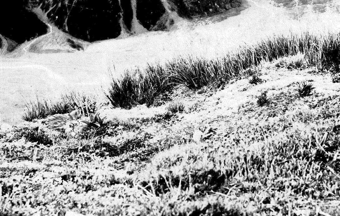Figure 18. Tahr camp in Chionochloa pallens grassland at 1700 m, Liebig Range; Murchison
River left background and Onslow Stream at top right (Photo: Hugh D. Wilson, 2 February 1971;
reproduced from Wilson 1976).

Wilson (1976) noted a shift in native dominance in response to local substantial reduction of
biomass of dominant Chionochloa spp. by tahr. He considered that Celmisia spp. (especially
C. lyallii) and Epilobium spp. had greater cover in these patches than in adjacent less heavily
grazed Chionochloa grasslands in Mount Cook National Park. Similarly, Wardle (1977, 1979)
considered Celmisia walkeri had greatly increased in cover in grasslands heavily grazed by
tahr in Westland National Park, along with the small herbs Hydrocotyle novae-zealandiae and
Anaphalioides bellidioides. Wilson (1976) also noted that there was recruitment of native
plant species that he thought were likely to have been dispersed to the sites by tahr (by
seeds that attach readily to fur, in the cases of Acaena hirsutula and Carex edura). We lack
analyses of the repeated-measures data from the subjectively located plots to determine
whether dominance shifts have occurred after tahr grazing, and we suggest that such
analyses and a wider community context would be profitable to evaluate Wilson’s (1976)
hypothesis.
In other grasslands, grazing by large mammalian herbivores exerts strong effects on soil
properties and soil biota, including through the fertilising effects of their urine and faeces
(Bardgett 2005; Harrison & Bardgett 2008). Alpine grasslands are often limited in their
productivity by availability of soil nutrients, especially nitrogen (e.g. Thébault et al. 2014). In
nitrogen-limited grasslands with an evolutionary history of mammal herbivory, large
mammalian herbivores have been shown to accelerate soil nitrogen cycling, alleviating
nutrient deficiency, and enhancing their own carrying capacity (McNaughton et al. 1997;
Frank et al. 2000). We do not know whether this is the case in New Zealand alpine grasslands
in which mammalian grazing is an evolutionary novelty. The effects of grazing by tahr of
alpine grasslands on the soil biota and properties is unknown, but if the effects are positive,
as is often the case (Bardgett 2005), then this could be a mechanism by which compensatory
growth occurs in heavily grazed patches. Studies are needed of the effects of tahr grazing on
- 42 -

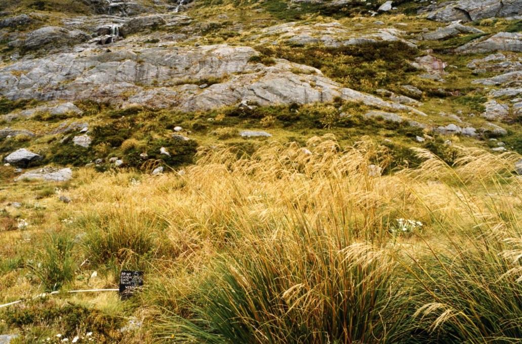
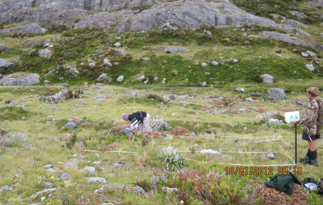
soil properties and biota, and whether alteration of belowground properties or induction of
positive feedbacks between grazing and plant responses is potentially a barrier to restoring
these habitats. Furthermore, if the local patches that are heavily grazed by tahr are induced
“grazing lawns” (McNaughton 1984), we know little about the long-term capacity for such
systems, which have not co-evolved with mammalian grazers, to be maintained, or whether
they may be fragile and disintegrate, exposing bare ground (already a feature of these sites,
Wilson 1976), if tahr densities increased substantially.

Figure 19. Vegetation in one of the 117 subjectively located plots (in Zora Creek, Westland) at
two points in time showing a reduction in tussock cover and height. Upper image in 1999; lower
in 2012 (photos provided by Ingrid Grüner, Department of Conservation, September 2018).

Tahr can also alter the structure and cover of alpine woody plant communities. Wilson (1976)
noted local-scale alteration of shrublands in Mount Cook National Park on steep, rocky,
north-facing slopes, which were “heavily browsed and battered” by tahr. Upper subalpine
shrublands were most affected, with Dracophyllum rosmarinifolium locally “completely
- 43 -

link to page 58
defoliated and often killed in a band up to 100 m wide visible from afar as a grey stripe
between scrub and alpine grassland” (Wilson 1976), yet such heavily impacted areas were
patchy within the National Park, occupying only a small area of the total proportion of
subalpine shrublands (Figure 20), mostly those on steep (>30º) slopes (Burrows 1974). In
Westland National Park, Wardle (1977) described areas of D. rosmarinifolium that had been
killed by tahr, and Wardle (1979) suggested shrublands dominated by Coprosma ciliata,
Olearia moschata and Polystichum vestitum browsed heavily by tahr can be replaced with
Hypolepis millefolium. There are long-term measurements of changes in subalpine
shrublands in response to browsing by red deer (Tanentzap et al. 2009), but there is no
equivalent study to that of Cruz et al. (2017) for subalpine shrublands heavily browsed by
tahr. Such studies are needed because shrubs such as D. rosmarinifolium are a key late-winter
food supply critical for the survival of tahr (an accessible food source through deep snow
drifts, Caughley 1970b; Wilson 1976; Tustin & Parkes 1988), and may therefore be key to
understanding the maximum densities of tahr that catchments could potentially support.
6.4  Disentangling drivers of change in the Ecological Integrity of alpine and
subalpine plant communities
Ecological Integrity was defined by Lee et al. (2005) through three components: indigenous
dominance, species occupancy, and ecosystem representation. The current definition of
ecological integrity covers 8 outcome objectives, of which we are concerned principally with 6
(we do not consider ‘limiting environmental contaminants’ and ‘human use and interaction
with natural heritage’ in this report). We argue below that the information basis for reporting
on these outcome objectives is weaker in subalpine and alpine ecosystems than it is in
forests, and provide suggestions for how this could be addressed. Importantly, we have only
a limited information base for disentangling the multiple drivers of change in alpine
ecosystems (cf. indigenous forests; Peltzer et al. 2014) and a more cohesive view of alpine
ecological integrity is required to underpin understanding and future reporting of tahr
impacts.
Maintaining ecosystem processes and Reducing spread and dominance of
exotic species
The extent to which ecological processes are dominated by native species will vary
throughout the alpine according to the abundance of non-native mammal species (tahr, as is
the focus of this report, plus the effects of other species shown in Fig. 6), non-native bird
abundance (e.g. introduced finches, which are likely to consume seeds of grasses, including
Chionochloa spp.), non-native plant abundance (e.g. many pastoral grasses are common in
alpine areas that were grazed historically), and cryptic non-native biota such as diseases.
The widespread distribution of many non-native herbivore species – including, of course, tahr
– raises the possibility that ecosystem processes associated with herbivory are not dominated
by native species. While the amount of herbivory by native species (e.g., grasshoppers, snails,
birds) could be substantial, the wider impacts of soil compaction and locally concentrated
faeces and urine are unique to larger-bodied herbivores and the resultant ecosystem
processes are novel and warrant further attention.
- 44 -

Non-native plant species are rarely dominant in alpine and subalpine ecosystems, although
there are striking exceptions, such as Hieracium lepidulum in the headwaters of Rob Roy
Stream, Mt Aspiring National Park. This contrasts with the induced non-forested communities
below the natural treeline. However, tahr – and other non-native herbivores – may disperse
non-native plant species beyond their current ranges, and further encourage their spread by
creating regeneration niches through localised disturbance and fertilisation with urine and
faeces. Turf-forming non-native grass species (e.g. Agrostis capillaris) are likely to be more
browse-resilient and encouraged by browsing. While diminutive in terms of biomass, these
non-native species have the potential to alter soil properties (Peltzer et al. 2009) and exclude
native species at local scales.
Maintaining ecosystem composition and Preventing declines and extinctions
Because of the selective nature of most herbivores, some species are likely to be locally
extirpated or greatly reduced in abundance by repeated browsing (potentially including
those selected for measurement as indicators of tahr grazing; McKay & McNutt 2016).
Sparrow & Kelly (2000) observed that “Thus quite rare plant species can be most palatable
and most susceptible to browsing. Such species can be the best indicators of vegetation
condition’ if condition is a measure of biodiversity of species rather than maximum biomass”.
Identifying these taxa and the settings in which they are selected (e.g. a species in a habitat at
a time of the year) will be important for determining whether highly preferred species are
being maintained across the full range of potential sites.
In forested ecosystems, there are abundant quantitative data spanning many decades that
can be used to define the potential distribution of many common forest species. We lack this
information in the alpine and this limits our capacity to determine whether current plant
distributions are a reasonable baseline for future monitoring, or whether they bear the
imprint of many decades of herbivory (i.e. many species are now restricted to habitats that
are atypical or have been promoted by herbivory). Wider sampling (Fig. 17) and syntheses of
existing vegetation data (e.g. species distribution models, habitat models) alongside
experimental manipulations (e.g. Grüner & Norton 2006) would provide an essential
foundation on which to report on and interpret change in alpine ecosystems.
Species may persist at sites but may be vastly altered in structure and function. Structurally,
local dominance by long-lived woody plants such as Dracophyllum can be reduced by tahr
with potential consequences for soil stability and regeneration of other species, and the rate
of recovery of biomass of subalpine woody plants after disturbance is slow (e.g. Calder &
Wardle 1969). Functionally, seed and flower production may be greatly depressed by
herbivory as these tissues are rich in nitrogen and phosphorus. An experimental study of hare
browse on native brooms (Carmichaelia spp.) reported substantial losses of reproductive
tissues through browse (Grüner & Norton 2006). If also true of tahr, this could have strong
effects on plant regeneration and the balance between asexual and sexual reproduction of
plant species.
Lastly, while the social behaviour of tahr may drive concentrated activity in key sites (e.g.,
concentrations of nannies, etc.) and while environmental drivers may govern sites for intense
herbivory, it is possible that diffuse activity impacts strongly on highly preferred, rare species,
- 45 -

whereas intense activity alters local dominance of less preferred, common species. Robust,
targeted Tier 2 monitoring could focus on communities of highly preferred, rare species.
Ensuring ecosystem representation
As the alpine is almost exclusively protected as Public Conservation Land, we consider that all
alpine ecosystems are likely to be protected. However, tahr extend on to private land. An
assessment of representation outside the publicly managed alpine ecosystems can only be
achieved once defined ecosystem types are mapped for the tahr management and exclusion
zones. Vegetation types are commonly used as surrogates for ecosystems (Affeld et al. 2018)
so augmenting existing vegetation classifications (e.g. Wiser et al. 2016), in combination with
fine divisions in LENZ (Leathwick et al. 2003) to address data gaps, and then mapping those
vegetation types across the management and exclusion zones would be needed to assess
whether a full range of ecosystem types are being maintained across the area.
Adapting to climate change
Changing climate regimes are forecast to have substantial, negative effects on the
distribution and integrity of alpine ecosystems. As McGlone & Walker (2011) stated, “Eventual
loss of much of the current alpine areas of New Zealand and severe reduction of cold-winter
habitat seems inevitable under even moderate scenarios for rising greenhouse gas
concentrations”. However, they further observed that “Overall, there is no basis for simplistic
assumptions about the results of warming on alpine organisms, and counter-intuitive
outcomes are possible”.
Responses to alpine and subalpine ecosystems to climate change are challenging to predict,
as is exemplified by the lack of response by New Zealand alpine treelines to warming over
last century (Harsch et al. 2009; Figure 1 in McGlone & Walker 2011). This may be because
the warming recorded so far is not occurring at a time of the year when tree recruitment
processes occur. Alternatively, it may be because periodic cold periods prevent treelines from
advancing, in spite of generally increasing mean annual temperatures. A richer understanding
of the spatial and temporal pattern of climate warming is needed to understand which
biological processes are most vulnerable to change. Changes in the extent of alpine
ecosystems are likely to be preceded by significant shifts in their composition, structure and
function. With regard to tahr impacts, the relationship between tahr themselves and climate
change is poorly understood. The consequences of warming, reduced snow cover and glacial
retreat for alpine plant phenology and composition can only be speculated on as the few
studies available point to slow, lagged or variable responses (e.g. Mark et al. 2015) and hence
the consequences for browsing behaviour are also unknown. In short, potential climate
change effects are highly uncertain and tahr browsing will be an additional driver of
vegetation change in alpine ecosystems as climates warm and become more variable.

- 46 -

6.5 Studies of long-term effects of tahr on alpine grasslands derive from
subjectively-placed plots
Since DOC is required to maintain ecological integrity across the tahr management zone, it is
important to determine the general inference that can be derived from the 117 subjectively
located plots. In a review of these plots, Sparrow and Kelly (2000) noted that “it is unclear
whether the clusters of [subjectively located] plots are indeed representative of whole
catchments”. Our analyses show that they are certainly not representative of the entire tahr
management zone. The subjectively placed plots are much wetter and receive much lower
sunshine hours than plots that representatively sample the tahr management zone. Whereas
alpine grasslands dominated by Chionochloa spp. represented 18% of the plots in non-
woody vegetation in an objective (Tier 1) sample in the tahr management zone, they
comprised 63% of the subjectively located plots. This is not surprising as a criterion for siting
the subjectively located plots was that a plot contained at least 20 Chionochloa individuals, a
condition that is not representative of Chionochloa abundance in the wider landscape. It is
unknown whether the subalpine shrublands that are heavily browsed by tahr at local scales
(Wilson 1976) are typical of subalpine shrublands throughout the tahr management and
exclusion zones; this information is needed to guide future Tier 2 monitoring work and
consequent management decisions.

- 47 -

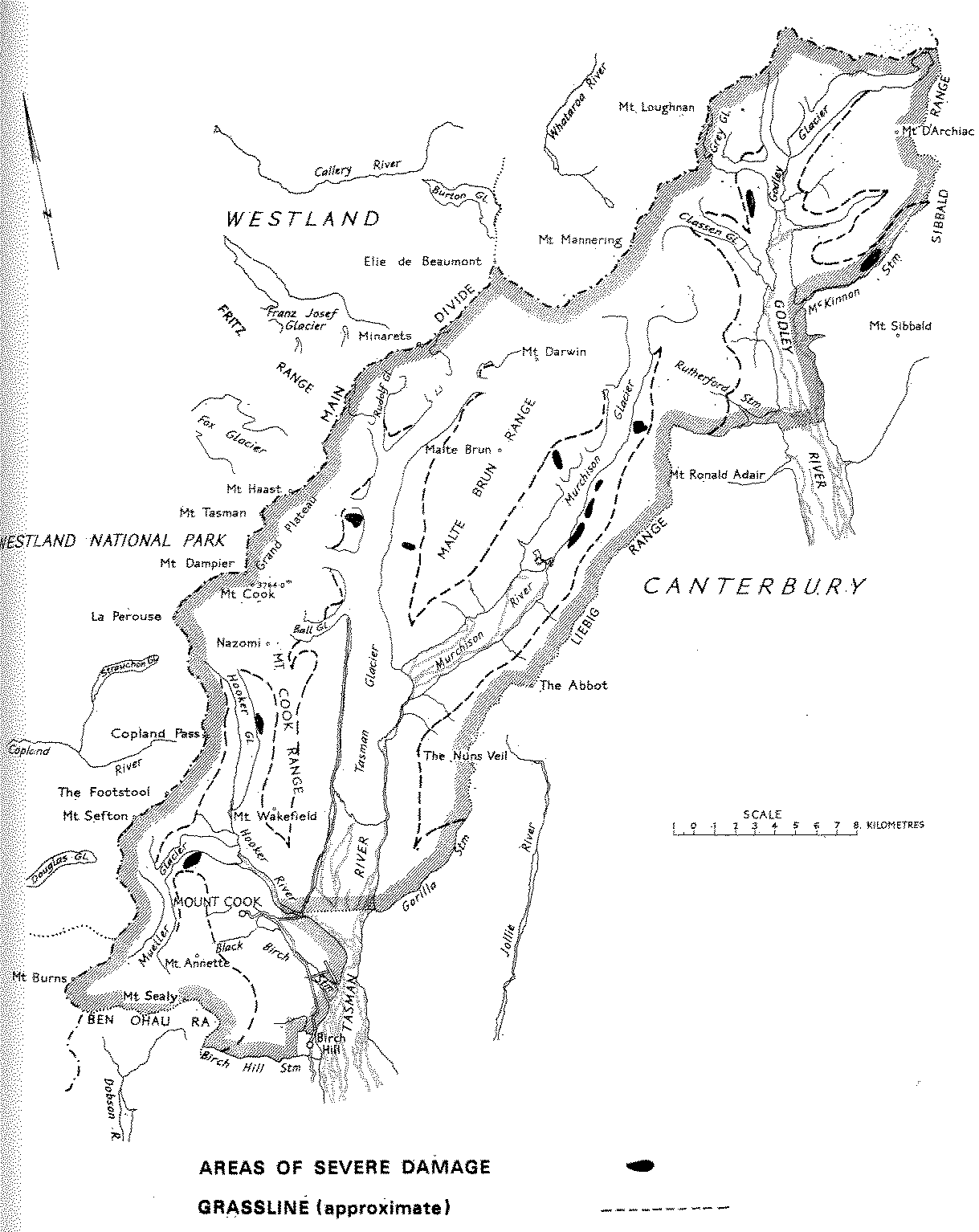Figure 20. Areas of severe damage to shrubland immediately below alpine grasslands in Mount
Cook National Park mapped in 1976 (reproduced from Wilson 1976).
6.6 Evaluating the suitability of current methods employed on Tier 1 plots to
assess changes in vegetation grazed by tahr
6.6.1 Whole-plot (20 × 20 m)
Relevés over the fixed area (400 m2) are recorded as a standard feature of Tier 1
methodology. The cover of all plant species is recorded in cover classes in fixed height tiers
(Hurst & Allen 2007). In alpine grasslands and many subalpine shrublands, cover data are
most likely to derive from only two height tiers, i.e. ≤0.3 m and 0.3–2 m. Whole-plot cover-
class values of dominant Chionochloa spp. are likely to be useful for assessing variability in
- 48 -

link to page 36 link to page 36 link to page 36
plot-level dominance and potentially for determining change in cover, but of no value in
assessing their patchiness within the plot. Plot-level cover for many plant species, especially
herbs, is likely to be low (cover classes ≤1%, or 1–5 %), and a widespread low-biomass
species will have the same cover class score regardless of it being a single individual or
multiple small individuals across the whole plot. The capacity for relevés to resolve change
with time in these species at the whole-plot scale is low.
Other means of assessing grassland and shrubland biomass can be achieved using height-
frequency methods (Scott 1965; Dickinson et al. 1992; Wiser & Rose 1997), and these have
been used recently in fixed area (100 m2) plots in tussock grasslands (Brownstein & Lee
2017). Nearest-neighbour-distance sampling (similar to the point-centred quarter sampling
method used in forests, Mueller-Dombois & Ellenberg 1974) is an efficient method for
estimating tussock density and mean tussock height and diameter using measurements from
only 16 individuals within a plot (Wiser & Rose 1997).
6.6.2 Sub-plot (5 × 5 m)
The total cover of each of the three indicator Chionochloa spp. (Table 4) is recorded in each
subplot (to the nearest 5%) and their heights are averaged across the subplot to the nearest
0.1 m. Compared with whole-plot estimates of cover, this is a substantial improvement in
assessing patchiness within the plot, which could be an early-warning indicator of tahr
impacts. However, we note that the coverage of Chionochloa species by this method is partial
– other species (e.g. C. crassiuscula, C. oreophila; Wilson 1976) that may co-occur are not
recorded. This method will result in more precise estimates of cover than whole-plot
estimates for three species, since actual covers per subplot can be summed across whole plot
(rather than assignment to sometimes broad cover-classes in the whole-plot relevé), and
recording heights to the nearest 0.1 m is a large improvement over two coarse height classes.
Although the visual estimates of tussock cover were not directly validated with independent
measurements of crown cover, their strong correspondence with projections of basal areas
(Fig. 10a) provides some confidence on the validity of visual estimates within subplots.
Counts of individual indicator species (per Table 4) and their cover and height are recorded in
each subplot as well. Conducting diligent searches per 25 m2 subplot will almost certainly
improve the quality of the obligatory whole-plot relevé, i.e. a relatively small investment in
time has major benefits for data quality.
We believe there is much merit in focusing on herbaceous species that are likely to be highly
palatable to tahr, i.e. the indicator species of Table 4, and many of these are of low
abundance and patchy in distribution (Sparrow & Kelly 2000). Data for indicator species could
be amenable to demographic interpretations, although some, e.g. Ranunculus lyallii, could
still achieve high density at 25-m2 scales, rendering demographic interpretations difficult.
Measuring the demography of herbaceous indicator species in these plots and subplots will
be problematic. Demographic data are best obtained from marked individuals (the equivalent
of tagged stems in forests), and attaching tags to some species will be difficult (especially for
R. lyallii, for which most aboveground parts arise each spring from a fleshy root stock).
Moreover, high mammalian herbivore densities (and perhaps kea, Nestor notabilis) would
probably destroy any attempts to mark individuals. We believe counts within subplots are
preferable to collecting demographic data at such large scales and sampling intensities as
Tier 1 plots.
- 49 -

link to page 36
Among the herbaceous indicator species, there are seven Aciphylla spp. (Table 4) and we
know little about the ecology of most of them (but see Campbell 1981 for A. aurea).
However, there is a large range among these species in their sizes (as rosettes and in height
of inflorescences; Mark 2012), habitats (Mark 2012), and ranges with respect to climate (Fig.
9), hence we encourage caution before “lumping” them or expecting them to have a uniform
response to tahr herbivory (cf. Peltzer et al. 2014). Many entangled factors are likely to be
driving the distribution and abundance of these indicator species, of which browsing is just
one. If each Aciphylla species was analysed separately, then just as is the case for two other
individual plant species used as indicators (Celmisia semicordata and Ranunculus lyallii), most
species are unlikely to occur on most plots, resulting in highly detailed count data at large
scale, but highly zero-inflated data (which reduces the statistical power of detecting
differences). This problem is likely to be resolved over time as more is learned about the
biology of these species, and how they can be grouped together based on their functional
responses to browsing. In the meantime, if measurements of these species entail little cost,
then we believe there is great merit in continuing to collect data.
Although Celmisia species are consumed by tahr (Tustin & Parkes 1988), the rationale for
including a single species (C. semicordata) among the many species in the region (e.g. 16
Celmisia spp. in Mount Cook National Park; Wilson 1976) as an indicator is unclear. Its
selection as an indicator species of tahr grazing in Tier 1 plots is presumably with an
expectation that tahr grazing would reduce, rather than promote, its biomass, yet two other
species may increase in abundance in response to intense tahr grazing of alpine grasslands
(C. lyallii, Wilson 1976; C. walkeri, Wardle 1977, 1979).
Counts of three Chionochloa spp. and their basal diameters and heights are measured,
noting the 5 × 5 m subplots in which they occur. In plots where these Chionochloa spp. are
sparse, the data are comprehensive but where they are dense, only some subplots are
measured. Measuring basal diameters yields size-class structures, which is a step towards
understanding the demography of individual Chionochloa species, i.e. we can infer that
recruitment of a species locally is continuous or episodic on the basis of frequency of
individuals in diameter classes, analogous to size-class structures for forest tree species. Since
little is known about the regeneration niches of most Chionochloa spp., this is valuable
information. Size-class structures, in terms of height and basal diameter, are described for C.
pallens, suggesting that this species recruits continuously at a landscape scale, but is reliant
on disturbed microsites (bare ground or reduced competition from surrounding vegetation)
for seedling recruitment at local scales (Rose & Platt 1990). Rose & Allen (1990) recorded
basal diameters in one group of the subjectively located plots in the tahr management zone,
but we note that they did not record basal diameters in one plot in which densities of C.
rigida were very dense. Currently, the lack of consistent sampling of Chionochloa spp. across
Tier 1 plots (comprehensive in some and not in others) hampers interpretation. We believe
that it is best to sample a consistent area within plots (of a size to be determined) within
which all Chionochloa species are measured comprehensively in order to obtain reliable
estimates of their size-class structures. Demographic data for them, as with the indicator
species, would be best derived from a tagging of all individuals within the same consistent
area, but this is time-consuming and could be compromised by the activities of mammalian
herbivores. As we recommend for herbaceous species, we believe counts within subplots is
preferable to collecting demographic data in non-woody Tier 1 plots.
- 50 -

link to page 52 link to page 36
We acknowledge that at local patches, Chionochloa spp. can be severely adversely affected
by tahr grazing, all but eliminating them (Figure 18; Wilson 1976; Wardle 1979), but this is so
far not widespread. Even in subjectively located plots in Chionochloa-dominated grasslands
that are favoured habitat of tahr, tussock heights remained little changed over nearly three
decades (Cruz et al. 2017) and similar to that of Tier 1 plots (note Cruz et al. do not report
change in cover of Chionochloa spp.). Caughley (1970c) noted that cover of Chionochloa spp.
was most sensitive to increasing densities of tahr and we recommend therefore that greater
emphasis is placed on measuring their cover (at whole-plot and subplot scales) in all future
measurements. Given that there have been significant changes in densities of tahr in some of
the catchments during that period, the lack of change in height with time suggests this is a
coarse indicator. Sparrow and Kelly (2000) questioned the emphasis on Chionochloa spp. in
the subjectively located plots because they considered them resilient to grazing (clearly up to
some threshold beyond which they are destroyed). We support their view. It is prudent to
maintain measurement of height and cover of the three Chionochloa spp. at subplot scales,
but we question the benefit of detailed measurements of basal diameter and other attributes.
These may be better suited to local, intense studies, including sites where current tahr
impacts are very intense.
7
Recommendations
1  Sampling vegetation browsed by tahr
a  Continue measurement of the subjectively located plots in tahr habitat,
emphasising cover of the three Chionochloa species, and including measurements of
the same indicator species listed in Table 4, since they provide the only longitudinal
data in the tahr management zone.
b  Establish a representative (Tier 2) vegetation plot network to increase power to
detect browsing effects, especially on individual plant species, with numbers of plots
as determined by power analyses (section 5.6). Tier 2 plots (together with Tier 1
plots) across tahr habitat can provide the data needed to determine the relative
abundance of each plant species for comparison with tahr rumen contents to
provide robustly chosen indicators of tahr impacts. These plots should include
measurements of individual Chionochloa species and herbaceous indicator species,
as on Tier 1 plots. The Tier 2 plot network needs to include historic plots with the
best time-series data, allowing interpretation of future change to build upon
documented historic change. An evaluation of the historic plots is therefore a critical
step before establishing a Tier 2 network.

Notable among the historic plots that sample the tahr management zone are those
in the Waitaki catchment where grassland ecosystems have been surveyed with
nearly 300 plots. These plots were installed in 1973/74 and remeasured in 1985/86
and hence describe vegetation at a time when tahr densities were probably much
lower than today. These plots use methods that have been applied in northern
Fiordland to quantify vegetation recovery after red deer control (Rose & Platt 1987)
so we recommend an immediate assessment of their potential to support Tier 2
monitoring, and their remeasurement. The design process for any Tier 2 network will
- 51 -

need to accommodate any reporting requirements in the tahr control plan
(Department of Conservation 1993).
c  Instigate long-term studies as measurements of Tier 3 (research) plots east and
west of the Main Divide of the Southern Alps in:
i
subalpine shrublands heavily browsed by tahr and maintain their
measurements, as has been conducted elsewhere (Murchison Mountains of
Fiordland; methods per Tanentzap et al. 2009). Collect environmental data from
these communities so that we can determine whether these are environmentally
distinctive, and to enhance prediction of where tahr impacts are likely to be
greatest in these communities.
ii  alpine grasslands heavily grazed by tahr. This is needed so that we can
identify these communities with confidence if they are widespread, or if they
become more common if tahr densities increase. Collect environmental data
from these communities so that we can determine whether these are
environmentally distinctive. If they are, then this could focus management on
areas at risk, and to target areas for restoration. More information within
management units is needed to determine whether the mosaic of locally highly
grazed patches of grassland are fixed or shift over time and whether, as
management-unit-level tahr densities are altered, whether this results in grazing
of previously less grazed sites.

Additionally, experimental studies (i.e. exclosures, which we acknowledge will
require constant maintenance in these environments) would reveal rates of
recovery of biomass and species composition in subalpine shrublands (cf.
Primack 1978) and alpine grasslands (cf. Rose & Platt 1992).
2  Methods on current plots
a  Maintain current additional measurements on Tier 1 plots at subplot (5 × 5 m)
scales including herbaceous indicator species, and including cover of the three
specified Chionochloa species at subplot scales.
b  Use constant areas within Tier 1 plots to quantify Chionochloa spp. Maintain
counts of the specified Chionochloa species within subplots. If size-class structures
(basal area measurements) are unfeasible across all plots (because it is too difficult
to distinguish all individuals), then we question the value of conducting partial
measurements.
c  Evaluate the suitability of height frequency methods and distance-based
tussock measurements. These should be evaluated in 400-m2 plots along a
gradient of tussock density alongside current methods, with each method timed in
the field. If they are quicker and yield equal or better data than current measures of
individual tussocks and cover, or if there are gains in statistical power from using
these methods, then DOC should consider adopting them instead. The comparability
of distance-based methods for tussocks vs. currently used ones in the subjectively
located plots (Cruz et al. 2017) also requires similar investigation (we note that both
methods determine height).

- 52 -

3  New research
a  Establish dietary preference of tahr using data from established and new plots to
match data about relative biomass of alpine and subalpine plant species to their
abundance (proportion of dry mass) in rumens (Parkes & Forsyth 2000).
b  Undertake a study of hare diet and dietary preferences throughout the alpine
and subalpine parts of the tahr management and exclusion zones since they are the
non-native mammal that is most frequent in the alpine zone (Norbury & Flux 2005;
Bellingham et al. 2016) and since it is more frequent than ungulates throughout the
tahr management and exclusion zones, east and west of the Main Divide of the
Southern Alps. Such a study is needed to better determine effects of mammal
herbivory in the zones and to better attribute effects of change to individual species.
c  Establish a ‘null model’ of ecological integrity in alpine and subalpine
ecosystems that includes the expected distributions and abundances of each
indicator species. In forested ecosystems, we understand that disturbance creates
canopy openings that favour the regeneration of palatable species (Peltzer et al.
2014). Hence, we incorporate covariates on stand structure into our comparisons of
palatable species abundance. We lack a similar framework for the alpine and we risk
attributing changes in species abundances to tahr, that are also being driven by
(among other things) fire, land use history, climate, climate change.
8
Acknowledgements
We thank Elise Arnst for assistance with data extraction from NVS; Richard Duncan for the R
routine to calculate potential solar radiation; Ingrid Grüner, Meredith McKay, Elaine Wright,
Dong Wang, and Kate McNutt for peer-review within the Department of Conservation; Bill
Lee for peer-review within Manaaki Whenua – Landcare Research; and Anne Austin for
editing the final report.
9
References
Affeld K, Wiser SK, Payton IJ, DeCáceres M 2018. Using classification assignment rules to
assess land-use change impacts on forest biodiversity at local-to-national scales. Forest
Ecosystems 5: 13.
Allen RB, Bellingham PJ, Wiser SK 2003. Developing a forest biodiversity monitoring approach
for New Zealand. New Zealand Journal of Ecology 27: 207–220.
Anderson MJ 2001. A new method for non-parametric multivariate analysis of variance.
Austral Ecology 26: 32–46.
Bardgett RD 2008. The biology of soil. Oxford, Oxford University Press.
Bellingham P, Mason N 2012. Utility of a permanent plot network to detect change in the
ecological integrity of forests in Ōhope Scenic Reserve, Bay of Plenty. Landcare
Research Contract Report LC1027 for Environment Bay of Plenty, Whakatāne.
- 53 -

Bellingham P, Richardson S, Gormley A, Monks A, Wiser S 2016 Department of Conservation
biodiversity indicators: 2016 fact sheets. Landcare Research Contract Report LC2973 for
Department of Conservation, Christchurch, New Zealand.
Brownstein GE, Lee WG 2017. Mt Ida Syndicate Pastoral Occupation Lease – biodiversity
monitoring report 2. Landcare Research Contract Report LC2804 for Department of
Conservation, Alexandra, and Mt Ida Syndicate, Ranfurly, New Zealand.
Burrows CJ 1974 A botanist’s view on the thar problem. Tussock Grasslands and Mountains
Institute Review 28: 5–18.
Calder JW, Wardle P 1969. Succession in subalpine vegetation at Arthur’s Pass, New Zealand.
Proceedings of the New Zealand Ecological Society 16: 36–47.
Campbell AD 1981. Flowering records for Chionochloa, Aciphylla, and Celmisia species in the
Craigieburn Range, South Island, New Zealand. New Zealand Journal of Botany 19: 97–
103.
Caughley G 1970a. Liberation, dispersal and distribution of Himalayan thar Hemitragus
jemlahicus in New Zealand. New Zealand Journal of Science 13: 220–239.
Caughley G 1970b. Fat reserves of Himalayan thar in New Zealand by sex, season, area, and
age. New Zealand Journal of Science 13: 209–219.
Caughley G 1970c. Eruption of ungulate populations with emphasis on Himalayan thar in
New Zealand. Ecology 51: 53–72.
Chapin FS, III, Follett JM, O’Connor KF 1982. Growth, phosphate absorption, and phosphorus
chemical fractions in two Chionochloa species. Journal of Ecology 70: 305–321.
Coomes DA, Allen RB, Scott NA, Goulding C, Beets P. 2002. Designing systems to monitor
carbon stocks in forests and shrublands. Forest Ecology and Management 164: 89–108.
Coomes DA, Allen RB, Forsyth DM, Lee WG. 2003. Factors preventing the recovery of New
Zealand forests following control of invasive deer. Conservation Biology 17: 450–459.
Crawley MJ 2007 The R book. Chichester, Wiley & Sons.
Cruz J, Thomson C, Parkes J 2014. Impact of Himalayan tahr (Hemitragus jemlahicus) on snow
tussocks in the southern Alps, New Zealand. Landcare Research Contract Report LC1900
for the Department of Conservation. 20 p.
Cruz J, Thomson C, Parkes JP, Grüner I, Forsyth DM 2017. Long-term impacts of an introduced
ungulate in native grasslands: Himalayan tahr (Hemitragus jemlahicus) in New Zealand’s
Southern Alps. Biological Invasions 19: 339–349.
De Cáceres M, Font X, Oliva F 2010. The management of numerical vegetation classification
with fuzzy clustering methods. Journal of Vegetation Science 21: 1138–1151.
Department of Conservation 1993. Himalayan thar control plan, Canterbury Conservancy,
Conservation Management Planning Series No 3. Christchurch, Department of
Conservation. 68 p.
Dickinson KJM, Mark AF, Lee WG 1992. Long-term monitoring of non-forest communities for
biological conservation. New Zealand Journal of Botany 30: 163–179.
Flux JEC 1967. Hare numbers and diet in an alpine basin in New Zealand. Proceedings of the
New Zealand Ecological Society 14, 27–33.
- 54 -

Forsyth DM 2000. Habitat selection and coexistence of the Alpine chamois (Rupicapra
rupicapra) and Himalayan tahr (Hemitragus jemlahicus) in the eastern Southern Alps,
New Zealand. Journal of Zoology 252: 215–225.
Forsyth DM, Coomes DA, Nugent G, Hall GMJ 2002. Diet and diet preferences of introduced
ungulates (Order: Artiodactyla) in New Zealand. New Zealand Journal of Zoology 29:
323–343.
Forsyth DM, Hickling GJ 1998. Increasing Himalayan tahr and decreasing chamois densities in
the eastern Southern Alps, New Zealand: evidence for interspecific competition.
Oecologia 113, 377–382.
Forsyth DM, Richardson SJ, Menchenton K 2005. Leaf chemistry predicts the diet preferences
of invasive red deer (Cervus elaphus) in a temperate New Zealand forest. Functional
Ecology 19: 495–504.
Forsyth DM, Tustin KG 2005. Himalayan tahr. In: King CM ed. The handbook of New Zealand
mammals, 2nd edn. South, Melbourne, Oxford University Press. Pp. 361–373.
Frank DA, Groffman PM, Evans RD, Tracy BF 2000. Ungulate stimulation of nitrogen cycling
and retention in Yellowstone Park grasslands. Oecologia 123: 116–121.
Green P, MacLeod CJ, Nakagawa S 2016. SIMR: an R package for power analysis of
generalized linear mixed models by simulation. Methods in Ecology and Evolution 7:
493-498.
Harrison KA, Bardgett RD 2008. Impacts of grazing and browsing by large herbivores on soils
and soil biological properties. In: Gordon IJ, Prins HHT eds The ecology of browsing and
grazing. Ecological Studies 195. Berlin, Springer. Pp. 201–216.
Harsch MA, Hulme PE, McGlone MS, Duncan RP 2009.Are treelines advancing? A global
metaanalysis of treeline response to climate warming. Ecology Letters 12: 1040–1049.
Holdaway RJ, Rose AB, Newell CL, Carswell FE 2014. Demographic drivers of biomass carbon
recovery in degraded perennial tussock grassland, with and without domestic grazing.
New Zealand Journal of Ecology 38: 201–212.
Hurst JM, Allen RB 2007. The Recce method for describing New Zealand vegetation – field
protocols. Lincoln, Manaaki Whenua – Landcare Research.
Kaufmann MR, Weatherred JD 1982. Determination of potential direct beam solar irradiance.
Forest Service Research Paper. Fort Collins, CO, USA, USDA. Pp. RM-242.
Keesing F 2000. Cryptic consumers and the ecology of an African savanna. Bioscience 50:
205–215.
Leathwick J, Morgan F, Wilson G, Rutledge D, McLeod M, Johnston K 2003. Land
Environments of New Zealand: Technical Guide. Auckland, David Bateman.
Lee W, McGlone M, Wright E comps 2005. Biodiversity Inventory and Monitoring: A review of
national and international systems and a proposed framework for future biodiversity
monitoring by the Department of Conservation. Landcare Research Contract Report
LC0405/122. 216 p.
Lee WG, Fenner M, Loughnan A, Lloyd KM 2000. Long‐term effects of defoliation: incomplete
recovery of a New Zealand alpine tussock grass, Chionochloa pallens, after 20 years.
Journal of Applied Ecology 37: 348–355.
- 55 -

Mark AF 2012. Above the treeline. A nature guide to alpine New Zealand. Nelson, Craig
Potton.
Mark AF, Korsten AC, Guevara DU, Dickinson KJM, Humar-Maegli T, Michel P, Halloy SRP,
Lord JM, Venn SE, Morgan JW, Whigham PA, Nielsen JA 2015. Ecological responses to
52 years of experimental snow manipulation in high-alpine cushionfield, Old Man
Range, south-central New Zealand. Arctic, Antarctic, and Alpine Research 47: 751–772.
McGlone MS, Walker S 2011. Potential effects of climate change on New Zealand’s terrestrial
biodiversity and policy recommendations for mitigation, adaptation and research.
Science for Conservation 312. Wellington, Department of Conservation.
McKay M, McNutt K. 2016. Tier 1 vegetation monitoring – Tahr browse impacts protocol.
Version 1.0. DOC-2664865.
McNaughton SJ 1984. Grazing lawns: animals in herds, plant form, and coevolution. American
Naturalist 124: 863–886.
McNaughton SJ, Banyikwa FF, McNaughton MM 1997. Promoting of the cycling of diet-
enhancing nutrients by African grazers. Science 278: 1798–1800.
Mueller-Dombois D, Ellenberg H 1974. Aims and methods of vegetation ecology. New York,
John Wiley & Sons.
Norbury G, Byrom A, Pech R, Smith J, Clarke D, Anderson D, Forrester G 2013. Invasive
mammals and habitat modification interact to generate unforeseen outcomes for
indigenous fauna. Ecological Applications 23: 1707–1721.
Norbury G, Flux JEC 2005. Brown hare. In: King CM ed. The handbook of New Zealand
mammals. 2nd edn. South Melbourne, Oxford University Press. Pp. 151–158.
Norton DA, Young LM 2016. Effects of sheep grazing exclusion on alpine tall tussock
grasslands. New Zealand Journal of Ecology 40: 179–185.
Oksanen J, Blanchet FG, Kindt R, Legendre P, Minchin PR, O'Hara RB, Simpson GL, Solymos P,
Stevens MHH, Wagner H 2013. vegan: Community Ecology Package. R package version
2.0-10. https://CRAN.R-project.org/package=vegan
Parkes JP, Forsyth DM 2008. Interspecific and seasonal dietary differences of Himalayan thar,
chamois and brushtail possums in the central Southern Alps, New Zealand. New
Zealand Journal of Ecology 32: 46–56.
Parkes JP, Thomson C 1995. Management of tahr. Part I: Tahr – vegetation – harvest model
development. Part II: Diet of tahr, chamois, and possums. Science for Conservation 7. 42
p.
Peet RK, Roberts DW 2013. Classification of natural and semi-natural vegetation. In: van der
Maarel E, Franklin J eds Vegetation ecology. New York, Oxford University Press. Pp. 28–
70.
Peltzer DA, Allen RB, Bellingham PJ, Richardson SJ, Wright EF, Knightbridge PI, Mason NWH
2014. Disentangling drivers of tree population size distributions. Forest Ecology and
Management 331: 165–179.
Peltzer DA, Bellingham PJ, Kurokawa H, Walker LR, Wardle DA, Yeates GW 2009. Punching
above their weight: low‐biomass non‐native plant species alter soil properties during
primary succession. Oikos 118: 1001–1014.
- 56 -

Pirie MD, Lloyd KM, Lee WG, Linder HP 2010. Diversification of Chionochloa (Poaceae) and
biogeography of the New Zealand Southern Alps. Journal of Biogeography 37: 379–
392.
Primack RB 1978. Effects of grazing on indigenous shrubs in tussock grassland at Cass,
Canterbury, New Zealand, New Zealand Journal of Botany 16: 461–469.
R Core Team 2017. R: A language and environment for statistical computing. Vienna, R
Foundation for Statistical Computing. https://www.R-project.org/.
Richardson SJ, Holdaway RJ, Carswell FE. 2014. Evidence for arrested successional processes
after fire in the Waikare River catchment, Te Urewera. New Zealand Journal of Ecology
38: 221–228.
Rose AB, Allen RB 1990. Impact of Himalayan thar on vegetation of the North Branch, Godley
Valley, Canterbury. Forest Research Institute Contract Report FWE90/32 for Department
of Conservation, Wellington.
Rose AB, Platt KH 1987. Recovery of northern Fiordland alpine grasslands after reduction in
the deer population. New Zealand Journal of Ecology 10: 23–33.
Rose AB, Platt, KH 1990. Age-states, population structure, and seedling regeneration of
Chionochloa pallens in Canterbury alpine grasslands, New Zealand. Journal of
Vegetation Science 1: 89–96.
Rose AB, Platt, KH 1992. Snow tussock (Chionochloa) population responses to removal of
sheep and European hares, Canterbury, New Zealand. New Zealand Journal of Botany
30: 373–382.
Schauber EM, Kelly D, Turchin P, Simon C, Lee WG, Allen RB, Payton IJ, Wilson PR, Cowan PE,
Brockie RE 2002. Masting by eighteen New Zealand plant species: the role of
temperature as a synchronizing cue. Ecology 83: 1214–1225.
Scott D 1965. A height frequency method for sampling tussock and shrub vegetation. New
Zealand Journal of Botany 3: 253–260.
Smale MC, Hall GMJ, Gardner RO 1995. Dynamics of kanuka (Kunzea ericoides) forest on
South Kaipara spit, New Zealand, and the impact of fallow deer (Dama dama). New
Zealand Journal of Ecology 19: 131–141.
Solly LD 1998. Responses in the genus Chionochloa to grazing by indigenous and exotic
vertebrate herbivores: an evaluation of seven low-alpine snow tussock taxa in south-
western South Island, New Zealand. Unpublished PhD dissertation, University of Otago,
Dunedin, New Zealand.
Sparrow A, Kelly D 2000. Thar density and vegetation condition. Conservation Advisory
Science Notes 281: 1–5.
Tanentzap AJ, Burrows LE, Lee WG, Nugent G, Maxwell JM, Coomes DA 2009. Landscape‐level
vegetation recovery from herbivory: progress after four decades of invasive red deer
control. Journal of Applied Ecology 46: 1064–1072.
Tanentzap AJ, Lee WG, Coomes DA 2012. Soil nutrient supply modulates temperature‐
induction cues in mast‐seeding grasses. Ecology 93: 462–469.
Thébault A, Clément JC, Ibanez S, Roy J, Geremia RA, Pérez CA, Buttler A, Estienne Y, Lavorel S
2014. Nitrogen limitation and microbial diversity at the treeline. Oikos 123: 729–740.
- 57 -

Thompson S, Grüner I, Gapare N. 2004. New Zealand Land Cover Database, version 2–
Illustrated guide to target classes. Wellington, Ministry for the Environment.
Thomson C, Parkes JP, Coleman MC, McGlinchy A 1997. Impact of Himalayan thar on alpine
tussock in the Hooker Valley and the North Branch of the Godley Valley. Landcare
Research Contract Report LC9697/97 for Department of Conservation, Wellington.
Tustin KG, Parkes JP 1988. Daily movement and activity of female and juvenile Himalayan thar
(Hemitragus jemlahicus) in the eastern Southern Alps, New Zealand. New Zealand
Journal of Ecology 11: 51–59.
Vinton MA, Burke IC 1995. Interactions between individual plant species and soil nutrient
status in shortgrass steppe. Ecology 76: 1116–1133.
Walker S, Steel JB, Rapson GL, Roxburgh SH, King WMcG, Watkins AJ, Myers TE, Keogh JA,
McQueen AAM, Wilson JB 2001. A Chionochloa/Sphagnum/cushion valley bog in east
Otago, New Zealand. New Zealand Journal of Ecology 25: 39–52.
Wang Y, Naumann U, Wright ST, Warton DI 2012. mvabund– an R package for model‐based
analysis of multivariate abundance data. Methods in Ecology and Evolution 3: 471–474.
Wardle P 1977. Plant communities of Westland National Park (New Zealand) and
neighbouring lowland and coastal areas. New Zealand Journal of Botany 15: 323–398.
Wardle P 1979. Plants and Landscape in Westland National Park. National Parks Authority
Scientific Series No. 3. Wellington, Department of Lands and Survey.
Warton DI, Foster SD, De’ath G, Stoklosa J, Dunstan PK 2015. Model-based thinking for
community ecology. Plant Ecology 216: 669–682.
Williams PA 1975. Studies of the tall-tussock (Chionochloa) vegetation/soil systems of the
southern Tararua Range, New Zealand. 2. The vegetation/soil relationships. New
Zealand Journal of Botany 13: 269-303.
Wilson HD 1976. Vegetation of Mount Cook National Park, New Zealand. National Parks
Authority Scientific Series No. 1. Wellington, Department of Lands and Survey.
Wiser SK, De Cáceres M 2013. Updating vegetation classifications: an example with New
Zealand's woody vegetation. Journal of Vegetation Science 24: 80–93.
Wiser SK, Hurst JM, Wright EF, Allen RB 2011. New Zealand’s forest and shrubland
communities: a quantitative classiﬁcation based on a nationally representative plot
network. Applied Vegetation Science 14: 506–523.
Wiser SK, Rose AB 2007. Two permanent plot methods for monitoring changes in grasslands:
a field manual. Lincoln, Manaaki Whenua – Landcare Research.
Wiser SK, Thomson FJ, De Cáceres M 2016. Expanding an existing classification of New
Zealand vegetation to include non-forested vegetation. New Zealand Journal of
Ecology 40: 106–178.
Wong V, Hickling GJ 1999. Assessment and management of hare impact on high altitude
vegetation. Science for Conservation 116. Wellington, Department of Conservation. 40
p.

- 58 -

Appendix 1. Correlation between environmental variables
Table A1. Pearson correlation coefficients between environmental variables across all Tier 1 and
subjectively located plots

.
rc
s y

pe
da
io
th 0

s
icit
y
t
5
f

p.
n
ra
rs
de
ion
m
da

t
e
io
a
t
e
PET
ou
re
l
e
at
h
u
di
a
gr
di
o t
e
ra
u

ra
l
in
oist
r

n
de
al
la
g
r
f
sh
m
de
an
la
l
n
so
u
in
al
t
slope
so
f
i
an

.
Rain
Su
Soil
an
lt
e
row
e
A
M
G
Plot
Pot
Rain
log
log
log
M
Mean annual temp.
–0.80

Growing degree days
–0.79
0.96

Plot slope
0.26  –0.22  –0.24

Pot. solar radiation
0.03  –0.12  –0.13  –0.15

Rainfall
0.00
0.08
0.12
0.00  –0.13

log Rainfall to PET ratio
0.27  –0.25  –0.20
0.09  –0.10
0.91

log Sunshine hours 50th perc.
–0.25
0.19
0.18  –0.05
0.11  –0.77  –0.85

log Soil moisture deficit days
–0.04  –0.04  –0.04  –0.07
0.12  –0.85  –0.84
0.67

Mean solar radiation
–0.20
0.14
0.16  –0.11
0.05  –0.57  –0.69
0.71
0.61
Mean 9am rel. humidity
0.04  –0.05  –0.07
0.10  –0.09
0.39
0.49  –0.33  –0.48  –0.72

- 59 -

Appendix 2. Further notes on assignation of plots to the noise class
We felt it most appropriate to assign new plots using the same values for ‘m’ and ‘distance to
noise’ as was used to create the classification in the first place. Although the average
composition (centroids) of the original clusters would be unchanged, changing these values
would change the variability around those centres from the original, thus changing the
concepts of the vegetation types defined and we wanted to assign the 208 plots to the
existing concepts. Initially we used a different defuzzification approach where we ignored the
Noise class and assigned all of the 208 plots to the alliance to which they had the highest
fuzzy membership value, even if this value was quite low. We found these results to be
nonsensical, with plots being inappropriately assigned to vegetation types that do not even
occur in the region.
We could have developed a more complex defuzzication rule where we had a target of say
5% of the 208 plots being assigned to the outlier class, or overrode assignment to the outlier
class if the fuzzy membership to a vegetation type was over some threshold value (e.g. 0.3).
However, we felt any such choice would be more arbitrary than the choice we did make. A full
sensitivity analysis (such as was done in Wiser SK, De Cáceres M. 2015. Sensitivity of a NZ
woody classification to specific analytical choices. Landcare Research Contract Report LC2249
prepared for the Department of Conservation) is beyond the scope of the current report.
In any case, we feel it is unlikely that changing these choices would have changed the
fundamental conclusion that the subset of the 208-plot dataset comprising the subjectively
located plots is compositionally biased when compared with the objectively located Tier 1
plots. Also, given that most of the 208 plots that were assigned are non-woody, the
proportion of plots designated as outliers is consistent with the original non-woody
classification. In the Discussion of this report we raise the point that the current national non-
woody classification is not as comprehensive as would be ideal for this analysis because of
the limited sampling to date in non-woody vegetation, particularly high-alpine areas. If the
base classification for assignment were more comprehensive, this would reduce the number
of plots assigned to the outlier class.

- 60 -

Appendix 3. Diagnostic plots for the NMS ordination
i
Scree plot to determine the number of axes. The horizontal line shows a stress
of 0.2, below which an NMS solution can be considered satisfactory (McCune &
Grace 2002).
0.4
0.3
s
s
ert 0.2
S
0.1
0
0
1
2
3
4
5
6
7
8
9
Number of axes

ii Shepard plot of ordination distances against original dissimilarities. Plot shows
two goodness of fit statistics: one, a nonmetric fit based on stress; the other, a
linear fit between fitted values and ordination distances.

- 61 -

Appendix 4. Diagnostic checks for propensity scoring analysis
Propensity scoring with the “es.mean” method resulted in satisfactory balancing of samples.
For most covariates, differences in standardized effect size between groups were reduced or
substantially reduced after sample weighting (blue lines in Fig. A1), with three covariates
having only moderate increases in effect size after weighting (red lines). Significant
differences between groups disappeared after “es.mean” weighting for 7 of the 9 variables
that showed differences before weighting (red dots in Fig. A1).
Groups are imbalanced if group contrasts for many covariates have small p-values. Effective
sample weighting should increase those p-values and bring them closer to the values
expected if samples were randomly assigned to groups (which can be expected to have a
uniform distribution, Ridgeway et al. 2017). A QQ plot that compares the quantiles of the
observed p-values to the quantiles of the expected uniform distribution suggests satisfactory
balancing of samples, with observed p-values running acceptably close to the expected null
values (the oblique line in Fig. A2).

es.mean.ATT
ks.max.ATT
ce
n
er 0.8
effid dr 0.6
a
d
n
a 0.4
st etul 0.2
so
b
A 0.0
Unweighted Weighted
Unweighted Weighted

Figure A1. Differences between sample groups before and after sample weighting based on
each of two propensity scoring methods, mean effect size (“es.mean”) and maximum
Kolmogorov-Smirnov distances (“ks.max”). Red dots indicate significant differences between
groups.

- 62 -

es.mean.ATT
ks.max.ATT
1.0
s
e 0.8
ul
va 0.6
-
p
st 0.4
et T 0.2
0.0
5
10
15
5
10
15
Rank of p-value for pretreatment variables
(hollow is weighted, solid is unweighted)

Figure A2. QQ plots for the p-values of group comparisons of covariates before and after
weighing (filled and open dots respectively) by each of two methods (mean effect size,
“es.mean”, and maximum Kolmogorov-Smirnov distances, “ks.max”). The oblique blue line
presents the corresponding quantiles of a uniform distribution and represents the expected null
hypothesis under random assignment of plots to treatment groups.

Ridgeway G, McCaffrey DF, Morral AR, Burgette L, Griffin BA 2017. Toolkit for weighting and
analysis of nonequivalent groups: a guide to the twang package. URL https://cran.r-
project.org/web/packages/twang/index.html [accessed 12 September 2018].

- 63 -

Appendix 5. Model diagnostics for environmental covariates
Diagnostic inspection of model residuals showed that residuals were generally balanced and
homogeneous across sample groups with some departure of homogeneity of variance for
Rainfall to PET ratio and Mean solar radiation (Fig. A3). We ran linear models and post-hoc
Tukey tests on ranked data for these two variables (the equivalent of non-parametric tests).
This transformation improved on homogeneity of variance (Fig. A4 below) and led to the
same differences between groups reported in Figure 5 in the main text, indicating that
models and tests were sufficiently robust to the moderate deviations from assumptions
found here.

Altitude
Mean annual temp.
Growing degree days
3
3
3
2
sl
sl
s
2
l
a
1
1
a
a
u
u
u
di
di
1
di
s
s
s
e
-1
-1
e
e
0
R
R
R
-3
-1
-3
1150
1200
1250
1300
5.4
5.6
5.8 6.0
6.2 6.4
550 600 650 700 750 800
Fitted values
Fitted values
Fitted values
Slope
Pot. solar radiation
Mean annual rainfall
3
1
2
sl
sl
sl
a
a
a
u
1
0
u
1
u
di
di
di
s
s
s
e
e
0
-1
e
R
-1
R
R
-1
-2
-3
-2
27.5
28.5
29.5
30.5
0.70
0.72
0.74
4500
5500
6500
Fitted values
Fitted values
Fitted values
log Rainfall to PET ratio
log Sunshine hours
log Soil moisture deficit days
4
3
sl
0
2
s
2
l
sl
.
a
a
a
1
u
u
u
d
1
i
di
di
s
0
s
s
0
e
e
0
.
e
R
R
0
R
-2
0.
-2
1-
0.90
1.00
1.10
1.20
3.10 3.12 3.14 3.16 3.18
0.5
0.6
0.7
Fitted values
Fitted values
Fitted values
Mean solar radiation
Mean relative humidity
3
2
2
sl
sl
a
1
1
a
u
u
di
0
di
s
0
s
e
e
R
R
-2
-2
12.55
12.65
12.75
80.4
80.8
81.2
81.6
Fitted values
Fitted values

Figure A3. Standardised residuals versus fitted responses for linear models fitted to
environmental covariates.
- 64 -

ranked Rainfall to PET ratio
ranked Mean solar radiation
150
150
sl
sl
a
50
a
u
50
u
di
di
s
0
s
e
5
0
-
e
5
R
R
-
0
0
5
5
1-
1-
100
120
140
160
120
130
140
150
160
Fitted values
Fitted values

Figure A4. Standardised residuals versus fitted responses for linear models fitted to ranked
environmental covariates.

- 65 -

Appendix 6. NVS vegetation information for the tahr management and
exclusion zones
The National Vegetation Survey databank (NVS) holds data from 3,388 unique plots in the
tahr management units and 1,270 unique plots in the tahr exclusion zones (Fig. 17).
The number of plots indicated for each survey includes those which are in the management
units and exclusion zones, not the total number of plots in the associated survey. Further
information is available from NVS (http://nvs.landcareresearch.co.nz).
National surveys
LUCAS and Tier 1 monitoring
The Land Use and Carbon Analysis System (LUCAS) and the National Biodiversity Monitoring
and Reporting System (Tier 1) measure and report on New Zealand’s carbon storage and
biodiversity. For native forest and shrubland vegetation a national grid-based network of
permanent plots is measured to provide an unbiased estimate of carbon storage and plant
biodiversity. Measurement began in 2002 and is ongoing. Within the tahr management areas
and exclusion zones there are 99 of these permanent plots, 21 of which have been
remeasured at least once.
National Forest Survey (NFS)
A nationwide survey of New Zealand’s forests was carried out to underpin the need for
management of the nation’s timber resource and to protect forest lands for other purposes.
NFS Westland was carried out between 1945 and 1956 and measures 12 plots in the area.
Crown Leasehold Monitoring Unit
These surveys provided an inventory of tussock grasslands in the South Island. Initially set up
in the 1970s–80s, large-scale re-measurements have been undertaken twice – once in the
early 1990s, and again in the mid-2000s.
•
BIRCHWOOD TRANSECTS (3 plots established in 1993; remeasured twice)
•
GLEN ROCK TRANSECTS (6 plots established in 1991; remeasured three times)
•
HUNTER VALLEY TRANSECTS 1985 (3 plots)
•
LOCHABER TRANSECTS (5 plots established in 1989; remeasured twice)
•
MT DOBSON TRANSECTS 1983 (3 plots)
•
WEST WANAKA TRANSECTS (15 plots established 1981; partially remeasured four
times)

- 66 -

Regional surveys
Permanent vegetation plots
Permanent plots are where fixed area plots or transects have been established, and the
vegetation has been measured precisely (e.g. tagged trees, sapling and seedling counts,
species lists). These are ideal for monitoring vegetation changes and the effects of
management. These surveys include:
•
ASPIRING FOREST 1977-1978
(123 plots)
•
ASPIRING GRASSLAND 1977-1978 (38 plots)
•
DINGLE BURN GRASSLAND 1976 (4 plots)
•
HAAST/ARAWATA FOREST 1970-1971 (8 plots)
•
HAAST/ARAWATA GRASSLAND 1970-1971 (21 plots)
•
HOKITIKA FOREST (21 plots established in 1957-1958; partially measured three times
with 27 additional plots measured in 1963)
•
HOKITIKA GRASSLAND (16 plots established in 1957-1958; remeasured twice plus
additional plots measured in 1963 and 1971 resulting in a total of 49 plots)
•
HOKITIKA MIXED 1971-1972 (54 plots)
•
HOKITIKA RIVER FOREST 1983-1986 (50 plots)
•
HOKITIKA/WHITCOMBE FOREST (116 plots established in 1982-1986; with one of
these being remeasured twice with the most recent measurement being 2009)
•
KARANGARUA/COPLAND (Westland National Park) FOREST (54 plots established in
1978-1979; partially remeasured three times, with the most recent measurement
being 2004)
•
LANDSBOROUGH 2008 (2 plots)
•
MFE CARBON TRANSECT 1998-1999 (6 plots)
•
New Zealand Next Generation Biodiversity Assessment (Phase 2) 2015 (1 plot)
•
NZ ADAPTIVE MANAGEMENT OF DEER FOREST 2006-2008 (26 plots)
•
RAKAIA FOREST 1979-1980 (29 plots)
•
RAKAIA/WILBERFORCE FOREST 1979 (38 plots)
•
RANGITATA FOREST 1978-1979
(25 plots)
•
THAR IMPACT SITE - ARBOR RIFT GRASSLAND (16 plots established 1992; partially
remeasured four times)
•
THAR IMPACT SITE - CARNEY'S CREEK GRASSLAND (20 plots established 1992;
partially remeasured three times)
•
THAR IMPACT SITE - FITZGERALD GRASSLAND (15 plots established 1999;
remeasured twice)
•
THAR IMPACT SITE - HOOKER GRASSLAND (9 plots established 1992; remeasured
twice)
•
THAR IMPACT SITE - NORTH BRANCH GRASSLAND (9 plots established 1990;
remeasured four times)
•
THAR IMPACT SITE – TOWNSEND (15 plots established in 1999; remeasured twice)
- 67 -

•
THAR IMPACT SITE - WHYMPER GRASSLAND (12 plots established 1993; partially
remeasured three times)
•
THAR IMPACT SITE – ZORA (15 plots established in 1999; remeasured twice)
•
WAIMAKARIRI GRASSLAND (2 plots established in 1961-1962; remeasured in 1972
and an additional plot measured)
•
WAITAKI FOREST 1973-1974 (55 plots established 1973-1974; partially remeasured
once)
•
WAITAKI GRASSLAND (342 plots established in 1973-1974; partially remeasured
once)
•
WESTLAND NATIONAL PARK GRASSLAND 1977-1978 (29 plots)
Exclosure plots
A number of surveys have set up paired exclosure and control plots to look at the impact of
deer and goat browsing on the vegetation, and also the impact of controlling these ungulate
populations. Surveys conducted include:
•
OHAU CANOPY GAPS AND EXCLOSURES 2006-2007 (5 plots; remeasured in 2013)
Other surveys
A number of other surveys have been carried out in the area which quantify the vegetation
within a fixed area at a given point in time but are not permanently marked. General
vegetation survey data include reconnaissance descriptions ('Recces') and are suitable for
vegetation descriptions, studies of species distributions, and studies needing only coarse
measurement of changes in vegetation. These surveys include:
•
ARROWSMITH FOREST 1985 (125 plots)
•
ASPIRING FOREST 1977-1978 (5 plots)
•
CANTERBURY HIGH COUNTRY HIERACIUM 2009  (60 plots)
•
CANTERBURY HIGH COUNTRY TUSSOCK GRASSLAND 2010-2011 (150 plots)
•
CARNEY'S CREEK MIXED 1991 (102 plots)
•
CRAIGIEBURN FOREST 1987-1989 (9 plots)
•
FOX RIVER FOREST 1982 (3 plots)
•
FRANZ JOSEF CHRONOSEQUENCE 2002 (1 plot)
•
GODLEY FOREST 1985 (1 plot)
•
HAAST/ARAWATA FOREST 1970-1971 (52 plots)
•
HAKATERE FOREST 1984-1985 (25 plots)
•
HOKITIKA FOREST 1957-1958 (1 plot)
•
HOKITIKA FOREST 1971-1972 (126 plots)
•
HOKITIKA RIVER FOREST 1983-1986 (57 plots)
•
HOKITIKA/WHITCOMBE FOREST 1982-1986 (38 plots)
•
MATHIAS FOREST 1989
(101 plots)
•
MCKENZIE MIXED 1984
(27 plots)
- 68 -

•
MFE CARBON TRANSECT MIXED 1998-1999 (1 plot)
•
Mount Cook National Park Botanical Survey MIXED 1968-1971 (544 plots)
•
Pastoral Lease Tenure Review Survey MIXED 2002-2007  (8 plots)
•
POERUA FOREST 1984-1985 (89 plots)
•
RAKAIA FOREST 1965-1967 (12 plots)
•
RAKAIA FOREST 1979-1980 (162 plots)
•
RAKAIA/MATHIAS FOREST 1986-1987 (311 plots)
•
RANGITATA FOREST 1975-1976
(47 plots)
•
RANGITATA FOREST 1978-1979
(1 plot)
•
S. W. M. E. P. MAHITAHI RIVER FOREST 1984-1985 (48 plots)
•
S. W. M. E. P. MOERAKI FOREST 1985
(36 plots)
•
S. W. M. E. P. PARINGA-OTOKO FOREST 1984-1985
(124 plots)
•
SOUTH ISLAND SHORT TUSSOCK GRASSLANDS 1960-1965
(4 plots)
•
TWO THUMB FOREST 1985  (111 plots)
•
UPPER WAITAKI BASIN RIVERBED GRASSLAND 2001-2003 (179 plots)
•
WAITAKI FOREST 1985-1986
(2 plots)
•
WANGANUI RIVER FOREST 1983-1984
(275 plots)
•
WESTLAND NATIONAL PARK FOREST 1977-1978  (109 plots)
•
WESTLAND NATIONAL PARK SCRUB 1977-1978  (18 plots)
•
WILLS VALLEY ECOLOGICAL SURVEY MIXED 2005  (14 plots)

- 69 -

Appendix 7. Relationship between ungulate and hare activity
Relationship between ungulate and hare activity based on frequency of faecal pellets. Note
that this does not account for the different areas of pellet plots.

0.1
8.0
stell 6.
e
0
p erah 4
.
.
q
0
erf
2.0
0.0
0.0
0.2
0.4
0.6
0.8
1.0
freq. ungulate pellets

- 70 -