ACT 1982
INFORMATION
RELEASED UNDER THE
OFFICIAL
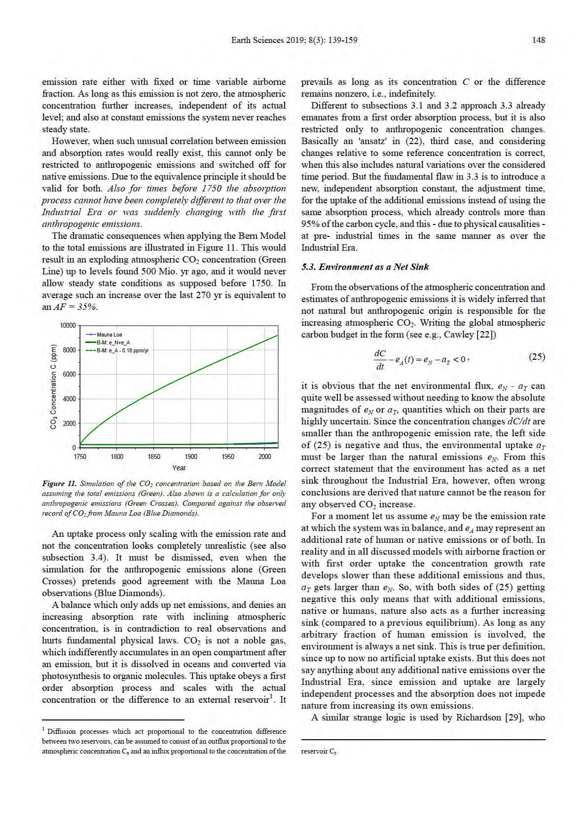
149
Hermann Harde: What Humans Contribute to Atmospheric CO2: Comparison of Carbon Cycle Models with Observations
considers mean values of the net atmospheric accumulation
reservoirs on atmospheric CO2, details of other extraneous
<
dC/dt> =
1.7 ppm/yr and of the human emissions <
dCA/dt> =
reservoirs of carbon are entirely irrelevant. This feature of the
eA(
t)
= 3 ppm/yr in a balance
governing physics is not only powerful, but fortunate.
Concerning carbonate chemistry, it is noteworthy that, in
dC /
dt −
dC /
dt
,
(26)
A
=
dC /
dt
N
< 0
the Earth’s distant past, CO2 is thought to have been almost
2000% as great as its present concentration (e.g., Royer et.
in which with <
dCA/dt> =
eA(
t) a priori any anthropogenic
al. [30]). Most of that was absorbed by the oceans, in which
absorptions are embezzled. From this relation it is also
carbon today vastly exceeds that in the atmosphere.
inferred that the average natural contribution <
dCN/dt> has
According to the IPCC, even in modern times the oceans
been to remove CO2 from the atmosphere, this with the same
account for 40% of overall absorption of CO2 (AR5 [1],
wrong conclusion as Cawley that the long term trend of rising
Fig.6.1). In relation to other sinks, their absorption of CO2
CO2 could not be explained by natural causes. This argument
is clearly not limited (see Appendix A). Of that 40%, over
is disproved with Figures 8 and 10. The fact that the
the Industrial Era anthropogenic CO2 represents less than
environment has acted as a net sink throughout the Industrial
1%. Contrasting with that minor perturbation in absorption
Era is a consequence of a dynamic absorption rate, which is
is oceanic emission of CO2. Through upwelling of
only controlled by the total CO2 concentration
C = CN + CA.
carbon-enriched water, the oceans significantly enhance
So, also with additional native emissions and/or temperature
natural emission of CO (Zhang [31]).
changes in the absorptivity the total uptake always tries - with
Different to our approach, which takes into account
some time delay - to compensate for the total emissions which,
human and also naturally varying emissions and
of course, also include the anthropogenic fraction. In other
absorptions, the models in Section 3 emanate from such a
words:
Since nature cannot distinguish between native and
simple and apparently flawed description that over
human emissions, nature is always a net sink as long as human
thousands of years CO2 was circulating like an inert gas in a
ACT 1982
emissions are not zero. Thus, except for shorter temporary
closed system, and only with the industrial revolution this
events like volcanic activities the environment will generally
closed cy le came out of control due to the small injections
act as a net sink even in the presence of increasing natural
by human emi sion .
emissions.
To equate <
dCA/dt> in (26) exclusively with human
5.5. Different Time Constants
emissions violates conservation of mass. Only when replacing
<
dC
The different time scales introduced with the models in
A/dt> by <
eA(
t)
- CA/τ
R>,
eq.(26) satisfies the Conservation
Law, and when additionally replacing <
dC
Section 3 represent different absorption processes for the
N/dt> by <
eN(
t)
-
C
uptake of atmospheric CO2 molecules by the extraneous
N/τ
R> eq.(26) converts to (23).
Again we emphasize that a separate treatment of the native
reservoirs. From physical principles it is impossible that an
and human cycle with their respective concentrations
C
absorption process would differentiate between naturally and
A and
C
anthropogenically
emitted
molecules.
The
temporal
N is possible if and only if no contributions are missing and
the two balances are linked together in on rate equ tion with
absorption or sequestration - except for smallest corrections
only one unitary residence time.
due to isotopic effects - is for all molecules identical.
The absorption also cannot decline unexpectedly by more
5.4. Too Simple Model
than one order of magnitude with the begin of the Industrial
INFORMATION
Era or because of an additional emission rate of a few %.
Often climate scientists argue that ch nges of CO2 in the
Observations show that no noticeable saturation over recent
atmosphere cannot be understood without considering
years could be found (Appendix A).
RELEASED UNDER THE
changes in extraneous systems (see e.g., AR5 [1], Chap.6;
Oceans and continents consist of an endless number of
Köhler et al. [8]), and they characterize the Conservation Law
sources and sinks for CO2 which act parallel, emitting CO2
as a flawed 1-box description because, a single balance
into the atmosphere and also absorbing it again. In the same
equation would not account for details in other reservoirs. In
way as the different emission rates add up to a total emission,
particular, they refer to carbonate chemistry in the ocean,
the absorption rates with individual absorptivities α
i - and
where CO2 is mostly converted to bicarbonate ions. As only
each of them scaling proportional to the actual CO2
about 1% rema ns in the form of dissolved CO2, they argue
concentration - add up to a total uptake as a collective effect
that only this small fraction could be exchanged with the
OFFICIAL
atmosphere. Due to this so-called Revelle effect, carbonate
a = α
C
1
+α
C
2
+ ... +α
C
T
N
.
(27)
chemistry
would sharply limit oceanic
uptake
of
= α
( 1 + α2 + ... + α ) ⋅
C = α ⋅
C
N
R
anthropogenic CO2.
In regard to understanding changes of CO2 in the
Collective absorption thus leads to exponential decay of
atmosphere, changes in extraneous systems are only
perturbation CO2 at a
single rate
qualifiedly of interest. The governing law of CO2 in the
atmosphere (4) and in more elaborate form (23) is self
α = 1/τ = α
.
(28)
1 + α 2 + ... + α
R
R
N
contained. With the inclusion of the surface fluxes
eT(
t)
and
a
This decay rate is faster
than the rate of any individual sink
T(
t)
= C /τ
R(
t), which account for influences of the adjacent
Earth Sciences 2019; 8(3): 139-159
150
and it prevails as long as its concentration
C or its difference to
as the main drivers for the observed CO2 increase in the
external reservoirs remains nonzero (see: Harde [6]; Salby
atmosphere and also for the continuous climate changes over
[11]).
the past and present times.
The above behavior is a consequence of the Conservation
The various mechanisms, along with their dependence on
Law and in contrast to the Bern Model, where decay proceeds
temperature and other environmental properties, could not
at
multiple rates. A treatment of CO2 with a multiple
have remained constant during the pre-industrial era. This
exponential decay obeys the following:
inconsistency invalidates the fundamental assumption, that
natural emission and absorption during the pre-industrial
−α
t
α
α
1
−
t
2
−
t
C =
C e
10
+
C e
20
+ ... +
C e N
N 0
.
(29)
period did remain constant. Even less this is valid over the
=
C
Industrial Era, a period which is characterized by the IPCC as
1 +
C2 + ... +
CN
the fastest rise in temperature over the Holocene or even the
Then differentiation gives:
last interglacial.
So, the CO
dC
2 partial pressure in sea water approximately
= −α
C e−α
t
α
α
1
2
α
α
changes with temperature as (
pCO
1
10
−
C e−
t...
2
20
−
C e−
t
N
2)sw(
T) =
pCO2) w(
T0)*
dt
N
N 0
exp[
0.0433*(
T-T
= −α
(30)
0)] (see: Takahashi et al. [32]) and thus, an
C
α
α
1
1 −
C ...
2
2
−
C
N
N
increase of
1°C causes a pressure change of about
18 µatm,
≠ −(α α
α
1 +
2 + ... +
) ⋅
C
N
which amplifies the influx and attenuates the outflux. From
observations over the North Atlantic Ocean (see, Benson et al.
At multiple decay rates the corresponding sinks operate, not
[33]) it can be estimated that a pressure difference ∆
pCO2
collectively, but independently. After a couple of their decay
between the atmosphere and ocean of
1 µatm contributes to a
times, the fastest sinks become dormant. Overall decay then
flux change of δ
fin ≈
0.075 mol/m2/yr = 3.3 g/m2/yr. Therefore,
continues only via the slowest sinks, which remove CO2
with an Earth s surface of
320 Mio. km2 covered by oceans and
ACT 1982
gradually. It is for this reason that such a treatment leaves
a pressure change of ∆
pCO2 =
18 µatm, under conventional
atmospheric CO2 perturbed for longer than a thousand years
conditions the native influx from oceans to the atmosphere
(Figure 5). In contrast, the behavior required by the
already increases by ∆
fin ≈
19 Pg/yr or
2.4 ppm/yr for an
Conservation Law decays as fast or faster than that of the
ave age temperature incline of
1°C. An even stronger
fastest sink (see (28)).
variation can be expected for the land vegetation with an
The observed decay of 14C shows that the corresponding
increased decomposition and reduced uptake of CO2 at rising
absorption is determined by a single decay time and operates
temperature (Lee [34]; Salby [11]).
on a time scale of only about one decade (see Figure 5). This
Together this causes an incline of the atmospheric CO2 level
scale is the same for the natural carbon cycle as for the
which is larger than all apparent human activities, but its
anthropogenic cycle. Therefore, it is unrealistic to differentiate
contribution is completely neglected in the official accounting
between a residence time and different adjustment times
schemes.
In this context it should be noticed that due to re-emissions
Also melting permafrost and emissions of volcanoes on
of 14CO2 from extraneous reservoirs the real residence time of
land and under water as well as any emissions at earthquakes
14CO2 in the atmosphere as well as that of the other
are not considered. In addition, actual estimates of dark
isotopologues of CO2 can only be shorter, ev n shorter than a
respiration suggest that under global warming conditions
decade (for details see subsection 5.7.3 and App ndix B).
INFORMATION
whole-plant respiration could be around 30% higher than
existing estimates (Huntingford et al. [35]). This longer list of
5.6. Temperature Dependence
different native events and effects is completely embezzled in
RELEASED UNDER THE
According to (9) or (10) we see that with increasing
the favored IPCC models.
atmospheric concentration over the Industrial Era from 280 to
Equally inconsistent is the presumption that additional
400 ppm either the residence time must be increased with
uptake of anthropogenic CO2, which represents less than 1%
temperature from 3 to about 4 yr, or τ
of the total over the Industrial Era, has, somehow, exceeded
R is considered to be
constant and the total emissions were rising from 93 to about
the storage capacity of oceans and other surface and
130 ppm/yr, synchronously increasing the concentration. Both
sub-surface reservoirs, capacity which is orders of magnitude
these limiting cases are in agreement with a temperature
greater.
A reduced absorption is rather the consequence of
anomaly of about 1.2 °C over this period (see GISS [9]), when
global warming than of saturation. Due to Henry's law and its
OFFICIAL
we assume the maximum temperature coefficients βτ
= 0.74
temperature dependence not only the partial pressure in sea
yr/°C or β
water increases, but also the solubility of CO
e = 24 ppm/yr/°C. However, generally both
2 in water
temperature induced natural emissions as well as temperature
declines exponentially with temperature and, thus, reduces the
dependent absorptions together will dictate the inclining
CO2 uptake. Often is this effect incorrectly misinterpreted as
concentration in the atmosphere.
saturation caused by a limited buffer capacity and dependent
In any way, as we see from Figure 8, is the CO
on the concentration level. But here we consider an uptake
2
concentration dominantly empowered by the temperature
changing with temperature, as this is known for chemical
increase; with only one unique decay process not human
reactions, where the balance is controlled by temperature.
activities but almost only natural impacts have to be identified
How strongly the biological pump (see Appendix A) and

ACT 1982
INFORMATION
RELEASED UNDER THE
OFFICIAL
Earth Sciences 2019; 8(3): 139-159
152
item).
half of the emissions remained in the atmosphere since 1750"
Since the fossil fuel emissions have a leaner difference
and "
the removal of all the human-emitted CO2 from the
(δ13C)fuel-atm = -18 ‰ compared to the atmosphere, or
atmosphere by natural processes will take a few hundred
(δ13C)fuel-VPDB = -25 ‰ with respect to the international VPDB
thousand years (high confidence)" (see AR5 [1], Chap.
carbonate standard (Coplen [38]), the rising human emissions
6-Summary and Box 6.1) can be simply refuted by the isotope
over the 30 yr interval can only have contributed to a decline
measurements at Mauna Loa. If the
113 ppm CO2 increase
of ∆ = (δ13C)
×
fuel-atm 1.8% = -18‰×1.8% = -0.32 ‰ or a
since 1750 (28.8% of the present concentration of
393 ppm -
(δ13C)atm = -7.92‰ in 2010. Thus, the difference to -8.3‰,
average between 2007 and 2016) would only result from
which is more than 50%, in any case must be explained by
human impacts and would have cumulated in the atmosphere,
other effects.
the actual (δ13C)atm value should have dropped by ∆ =
One possible explanation for a faster decline of (δ13C)
×
atm to
(δ13C)fuel-atm 28.8% = -18‰×28.8% = -5.2‰ to (δ13C)atm ≈
-8.3‰ can be - even with oceans as source and an 13C/12C ratio
-7‰ -5.2‰ = -12.2‰, which by far is not observed. (δ13C)atm
in sea water greater than in air (particularly in the surface
in 1750 was assumed to have been -7‰.
layer) - that the lighter 12CO2 molecules are easier emitted at
the ocean's surface than 13CO
5.7.3. Fossil Fuels are Devoid of Radiocarbon
2, this with the result of a leaner
13C concentration in air and higher concentration in the upper
“Because fossil fuel CO2 is devoid of radiocarbon (14C),
water layer (see also: Siegenthaler & Münnich [39]). From
reconstructions of the 14C/C isotopic ratio of atmospheric
water we also know that its isotopologues are evaporated with
CO2 from tree rings show a declining trend, as expected
slightly different rates.
from the addition of fossil CO2 (Stuiver and Quary, 1981;
Such behavior is in agreement with the observation that
Levin et al., 2010) Yet nuclear weapon tests in the 1950s
with higher temperatures the total CO
and 1960s have been offsetting that declining trend signal
2 concentration in the
atmosphere increases, but the relative 13CO
by adding 14C to the atmosphere. Since this nuclear weapon
2 concentration
ACT 1982
decreases. This can be observed, e.g., at El Niño events (see:
induced 14C pulse in the atmosphere has been fading, the
1
M. L. Salby [40], Figure 1.14; Etheridge et al. [41]; Friedli et
C/C isotopic ratio of atmospheric CO2 is observed to
al. [42]).
resume its declining trend (Naegler and Levin, 2009;
We also remind at the Mauna Loa curve, which shows for
Graven et al., 2012).”
the total emissions a seasonal variation with an increasing CO2
For 14C we can adduce almost the same comments as listed
concentration from about October till May and a decline from
for 13C. Fossil CO2 devoid of 14C will reduce the 14C/C ratio of
June to September. The increase is driven by respiration and
the atmosphere, this is valid for our approach in the same
decomposition mainly on the Northern Hemisphere (NH) as
manner as for the IPCC schemes. But, as no specific
well as the temperature on the Southern Hemisphere (SH) and
accumulation of anthropogenic molecules is possible
also local temperature effects. The (δ13C)atm value is just
(equivalence principle), this decline can only be expected
anti-cyclic to the total CO2 concentration (AR5 [1], Figure
proportional to the fraction of fossil fuel emission to total
6.3) with a minimum at maximum CO2 concentration and with
emission. Before 1960 this was not more than 1% and actually
seasonal variations of 0.3 - 0.4‰, the same order of magnitude
it is about 4.3%.
as the fossil fuel effect.
14C is continuously formed in the upper atmosphere from
An increase of 13C in the upper strata of oceans also results
14N through bombardment with cosmic neutrons, and then
INFORMATION
from an increased efficiency of photosynthesis for lighter
rapidly oxidizes to 14CO2. In this form it is found in the
CO2. Plankton accumulates this form and sinks to lower
atmosphere and enters plants and animals through
layers, where it decomposes and after longer times is emitted
photosynthesis and the food chain. The isotopic 14C/C ratio in
RELEASED UNDER THE
in higher concentrations with stronger upwelling waters
air is about 1.2⋅10-12, and can be derived either from the
particularly in the Eastern Tropic Pacific. It is also known that
radioactivity of 14C, which with an average half-lifetime of
the 13C concentrations are by far not equally distributed over
5730 yr decays back to 14N by simultaneously emitting a beta
the Earth's surface. Thus it can be expected that with volcanic
particle, or by directly measuring the amount of 14C in a
and tectonic activities different ratios will be released.
sample by means of an accelerator mass spectrometer.
So, without any doubts fossil fuel emissions will slightly
Fossil fuels older than several half-lives of radiocarbon are,
dilute the 13CO2 conc ntration in air. But presupposing regular
thus, devoid of the 14C isotope. This influence on radiocarbon
conditions for the uptake process (equivalence principle) they
measurements is known since the investigations of H. Suess
OFFICIAL
contribute less than 50% to the observed decrease. The
[43] who observed a larger 14C decrease (about 3.5%) for trees
difference has to be explained by additional biogeochemical
from industrial areas and a smaller decline for trees from
processes. Particularly the seasonal cycles and events like El
unaffected areas. This so-called Suess or Industrial effect is
Niños are clear indications for a stronger temperature
important for reliable age assignments by the radiocarbon
controlled modulation of the (δ13C)atm value. Therefore is an
method and is necessary for respective corrections. But for
observed decline of the 13C/12C ratio over recent years by far
global climate considerations it gives no new information, it
not a confirmation of an anthropogenic global warming
only confirms the calculations based on the human to total
(AGW) theory.
emission rate (see above), and it clearly shows that an
Also the widely spread but wrong declaration that "
about
assumed accumulation of anthropogenic CO2 in the
153
Hermann Harde: What Humans Contribute to Atmospheric CO2: Comparison of Carbon Cycle Models with Observations
atmosphere contradicts observations.
completely sequestered beneath the Earth's surface by a single
More important for climate investigations is that after the
absorption process. A substantial fraction is therefore returned
stop of the nuclear bomb tests 1963 14C could be used as a
to the atmosphere through re-emission (e.g., through
sensitive tracer in the biosphere and atmosphere to study
decomposition of vegetation which has absorbed that 14C), and
temporal carbon mixing and exchange processes in the carbon
in average it takes several absorption cycles to completely
cycle. As the bomb tests produced a huge amount of thermal
remove that 14C from the atmosphere. This simply modifies
neutrons and almost doubled the 14C activity in the
the effective absorption for radiocarbon, but with a resulting
atmosphere, with the end of these tests the temporal decline of
decay which remains exponential (see Figure 5). Unlike any
the excess radiocarbon activity in the atmosphere can well be
dilution effect by fossil fuel emission, which is minor (see
studied. This decline is almost completely independent of the
Appendix B), this re-emission slows decay over what it would
radioactive lifetime, but practically only determined by the
be in the presence of pure absorption alone. Therefore is the
uptake through extraneous reservoirs.
apparent absorption time - as derived from the 14C decay curve
Such decline has already been displayed in Figure 5 as
- longer than the actual absorption time.
fractionation-corrected ‰-deviations ∆14CO2 from the Oxalic
In this context we emphasize that apart from some minor
Acid activity corrected for decay, this for a combination of
influence due to fractionation all CO2 isotopologues are
measurements at Vermunt and Schauinsland (Magenta Dots
involved in the same multiple re-emission cycles. But in (23)
and Green Triangles; data from Levin et al. [17]). The decay is
or (32) this is already cons dered in the total balance via the
well represented by a single exponential with a decay constant
emission rates, for which it makes no difference, if the same or
of about 15 yr (Dashed Blue). For similar observations see
meanwhile exchanged molecules
re recycled to the
also Hua et al. [18] and Turnbull et al. [19]. Thus, the decay
atmosphere. In contrast to this are 14CO2 isotopologues
satisfies the relation
identified through their radioactivity, and in the worst case
without any dilution or exchange processes in an external
ACT 1982
dC'
1
14 = −
⋅
C' ,
(31)
reservoir τ
14
14 would approach the radioactive lifetime. On the
dt
τ14
other h nd, at strong diffusion, dilution or sequestration of 14C
in such reservoirs τ
14 would converge to τ
R. Consequently it
where
C'14 represents the excess concentration of radiocarbon
fol ws from the observed 14C decay shown in Figure 5 that
above a background concentration in the atmosphere. It
this provides an upper bound on the actual absorption time τ
R,
corresponds to absorption that is proportional to instantaneous
which can be only shorter. Both are tremendously shorter than
concentration with an apparent absorption time τ
14 slightly
the adjustment time requested by the IPCC.
more than a decade.
The exponential decay of 14C with only one single decay
Because CO2 is conserved in the atmosphere it can change
time proves models with multiple relaxation times to be
only through an imbalance of the surface fluxes
eT and
aT. This
wrong. At the same time it gives strong evidence for a first
holds for all isotopologues of CO2 in the same way. For this
order absorption process as considered in Section 4.2
reason, its adjustment to equilibrium must proceed through
those influences. They are the same influences that determine
5.7.4. Higher Fossil Fuel Emissions in the Northern
the removal time of CO2 in the atmosphere. If CO2 is
Hemisphere
perturbed impulsively (e.g., through a transient spike in
“Most of the fossil fuel CO2 emissions take place in the
emission), its subsequent decay must track the removal of
industrialised countries north of the equator. Consistent
INFORMATION
perturbation CO2,
C', which in turn is proportional to its
with this, on annual average, atmospheric CO2
instantaneous concentration. Determined by the resulting
measurement stations in the NH record increasingly higher
RELEASED UNDER THE
imbalance between
eT and
aT, that decay is governed by the
CO2 concentrations than stations in the SH, as witnessed by
perturbation form of the balance equation:
the observations from Mauna Loa, Hawaii, and the South
dC'
1
Pole (see Figure 6.3). The annually averaged concentration
= −
⋅
C' ,
(32)
difference between the two stations has increased in
dt
τ
R
proportion of the estimated increasing difference in fossil
which is the same form as the observed decay of 14C following
fuel combustion emissions between the hemispheres (Figure
elimination of the pe turbing nuclear source. But there is still
6.13; Keeling et al., 1989; Tans et al., 1989; Fan et al.,
one important difference between these equations.
1999)”.
OFFICIAL
Eq.(32) is the perturbation form of (23) with a decay time
The strongest terrestrial emissions result from tropical
τ
R, the residence time, because
1/τ
R describes the rate at which
forests, not industrial areas. The strongest oceanic emissions
CO2 is removed from the atmosphere, this as the result of the
can be seen from the map of Takahashi et al. [32]. They are
balance between all absorption and emission processes.
In contrast to this describes (31) a decay process, which
implicitly also considers some back-pumping of radiocarbon
2 A calculation similar to Figure 8 but with a residence time of 15 yr as an upper
to the atmosphere (see Appendix B, (37)). So, from all 14C that
bound would require to reduce the natural emissions at pre-industrial times from
93
is removed from the atmosphere with the time constant τ
ppm/yr to
19 ppm/yr. Then the anthropogenic contribution would supply
59 ppm,
R - in
which is 15% of the total atmospheric concentration or 52% of the increase since
the same way as all isotopes -, only some smaller fraction is
1850.
Earth Sciences 2019; 8(3): 139-159
154
between 10°N and 10°S in the Eastern Tropic Pacific.
by a single balance equation, the Conservation Law (23),
Nevertheless, there is no doubt that industrial emissions
which considers the total atmospheric CO2 cycle, consisting of
endow their fingerprints in the atmosphere and biosphere
temperature and thus time dependent natural emissions, the
(Suess effect). The influence and size of these emissions has
human activities and a temperature dependent uptake process,
already been discussed above, and their different impact on
which scales proportional with the actual concentration. This
the two hemispheres can be estimated from Figure 6.3c of
uptake is characterized by a single time scale, the residence
AR5 [1] indicating a slightly faster decline of (δ13C)atm for the
time of about 3 yr, which over the Industrial Era slightly
NH in agreement with predominantly located industrial
increases with temperature. Only this concept is in complete
emissions in this hemisphere. Even more distinctly this is
conformity with all observations and natural causalities. It
illustrated by Figure 6.13 of AR5 [1] for the difference in the
confirms previous investigations (Salby [7, 10]; Harde [6])
emission rates between the northern and SH with 8 PgC/yr,
and shows the key deficits of some widespread but largely ad
which can be observed as a concentration difference between
hoc carbon cycle models used to describe atmospheric CO2,
the hemispheres of 3.8 ppm. But this is absolutely in no
failures which are responsible for the fatal conclusion hat the
dissent to our result in Section 4 that from globally
4.7 ppm/yr
increase in atmospheric CO2 over the past 270 years is
FFE and LUC (average emission over 10 yr) 17 ppm or 4.3 %
principally anthropogenic.
contribute to the actual CO2 concentration of
393 ppm
For a conservative assessment we find from Figure 8 that
(average). This impact is of the same size as seasonal
the anthropogenic contribu ion to the observed CO2 increase
variations observed at Mauna Loa before flattening and
over the Industrial Era is significantly less than the natural
averaging the measurements.
influence. At equilibrium this contribution is given by the
fraction of human to native impacts. As an average over the
5.7.5. Human Caused Emissions Grew Exponentially
period 2007-2016 the anthropogenic emissions (FFE&LUC
“The rate of CO2 emissions from fossil fuel burning and land
together) d nated not more than 4.3% to the total
ACT 1982
use change was almost exponential, and the rate of CO2
concentration of 393 ppm, and their fraction to the
increase in the atmosphere was also almost exponential and
atmospheric increase since 1750 of 113 ppm is not more than
about half that of the emissions, consistent with a large body of
17 ppm or 15%. With other evaluations of absorption, the
evidence about changes of carbon inventory in each reservoir
con ribution from anthropogenic emission is even smaller.
of the carbon cycle presented in this chapter”.
Thus, not really anthropogenic emissions but mainly natural
The size and influence of FFE and LUC on the atmospheric
processes, in particular the temperature, have to be considered
CO
as the dominating impacts for the observed CO
2 concentration has extensively been discussed in the
2 increase over
preceding sections. Only when violating fundamental physical
the last 270 yr and also over paleoclimate periods.
principles like the equivalence principle or denying basic
causalities like a first order absorption process with only a
Acknowledgements
single absorption time, the CO2 increase can be reproduced
with anthropogenic emissions alone.
The author thanks Prof. Murry Salby, formerly Macquarie
In contrast to that we could demonstrate that conform with
University Sydney, for many stimulating discussions when
the rising temperature over the Industrial Era and in
preparing the paper, and Jordi López Fernández, Institute of
conformity with all physical legalities the overwhelming
Environmental Assessment and Water Studies Barcelona, for
INFORMATION
fraction of the observed CO
his support when searching for temperature data.
2 increase has to be explained by
native impacts. Such simulations reproduce almost every
This research did not receive any specific grant from
detail of the observed atmospheric CO
funding agencies in the public, commercial, or not-for-profit
RELEASED UNDER THE
2 increase (see Figures 8
and 10). And from observations of natural emissions it can be
sectors.
seen that they are increasing slightly exponential with
temperature (Takahashi et al. [32]; Lee [34]).
Appendix
Thus, no one of the preceding lines of evidence can really
support the above statement that "
fossil fuel burning and land
Appendix A
use change are the dominant cause of the observed increase in
The absorption efficiency of extraneous reservoirs has been
atmospheric CO2 concentration." In fact, they apply in the
claimed to have decreased, based on changes in the
same way for our concept, and thus they are useless to
arbitrarily-defined airborne fraction (e.g., Le Quéré et al. [12];
OFFICIAL
disfavour our approach. The isotopic studies rather confirm
Canadell et al. [44]). Such claims are dubious because they
our ansatz of a first order absorption process with a single
rely on the presumption that changes of CO
absorption time, which is significantly shorter than one
2 are exclusively of
anthropogenic origin. Nor are the claims supported by recent
decade, and they refute the idea of cumulating anthropogenic
atmospheric CO
emissions in the atmosphere.
2 data. Gloor et al. [45] found that decadal
changes of AF followed from changes in the growth of
anthropogenic emissions - not from changes in absorption
6. Conclusion
efficiency, which were comparatively small. Further,
uncertainties in emission and absorption exceeded any
The increase of CO2 over recent years can well be explained
155
Hermann Harde: What Humans Contribute to Atmospheric CO2: Comparison of Carbon Cycle Models with Observations
changes in AF. Ballantyne et al. [46] arrived at a similar
atmosphere. Anthropogenic CO2 in surface water is then
conclusion. They used global atmospheric CO2 measurements
quickly removed. It is also well known that higher concen-
and CO2 emission inventories to evaluate changes in global
trations of CO2 magnify photosynthesis. At increased atmos-
CO2 sources and sinks during the past 50 years. Their mass
pheric CO2, the plankton community consumed 39% more
balance analysis indicates that net CO2 uptake significantly
DIC (Riebesell et al. [53]). During summer and autumn, sur-
increased, by about 0.18 Pg/yr (0.05 GtC/yr) and, between
face CO2 can rapidly increase to 1000 ppm - more than twice
1960 and 2010, that global uptake actually doubled, from 8.8
the concentration of CO2 in the atmosphere. Surface water
to 18.4 Pg/yr. It follows that, without quantitative knowledge
then significantly enhances natural emission to the atmos-
of changes in natural emission, interpretations based on AF
phere. Conversely, during winter, surface CO2 remains at
are little more than speculative.
about 340 ppm. Despite reduced photosynthesis, CO2 in
The uptake and outgassing of atmospheric CO2 by oceans is
surface water then remains below equilibrium with the
simulated with complex marine models. How much CO2
atmosphere, reflecting efficient removal through downward
enters or leaves the ocean surface is calculated from the
transport by the biological pump. It is noteworthy that these
difference between atmospheric and surface concentrations of
strong seasonal variations of CO2 in surface water are mani-
CO2, modified by the Revelle factor. However, most of these
fest in the record of atmospheric CO2 (see Figures 9 and 10).
models involve assumptions which are not in agreement with
Under steady state conditions, diffusion of CO2 into the
observed behavior (see, e.g., Steele [47]). They assume that
ocean is believed to require about 1 year to equilibrate with an
the surface layer absorbs CO2 through equilibrium with
atmospheric perturbation. But, when increased sunlight
atmospheric concentration. On this premise, they calculate
enhances photosynthesis, such equilibration is no longer
how much Dissolved Inorganic Carbon (DIC) will be added to
achieved. Perturbation CO2 is then simply transported to
the ocean based on increased atmospheric CO2 since pre-indu-
depth, where it is sequestered from surface waters
strial times. In reality, the surface layer is not at equilibrium
(McDonnell et al. [54]). Under such conditions uptake of CO2
ACT 1982
with the atmosphere. A difference in concentration results
is not restricted by the Revelle factor but by the biological
from conversion of CO2 into organic carbon by
pump.
photosynthesis. Organic carbon produced then sinks into the
The foregoing processes are controlled essentially by
deep ocean, where it is sequestered. This downward transport
sunlight and temperature. There is no reason to believe that net
to the deep ocean is known as the biological pump. In the
primary production, the biological pump, and sequestration of
Northeastern Atlantic basin, e.g., Benson et al. [33] report on
CO2 below surface waters would be the same today as 270
seasonal pressure differences between the ocean and
years ago, when temperature and atmospheric CO2 were likely
atmosphere of ∆
pCO2 = -70 µatm and an air-sea CO2 flux
of
lower.
220 g/m2/yr. Only in those regions where strong upwelling of
In simulating transport of carbon in the ocean, complex
DIC from the deep ocean exceeds sequestration of carbon via
models assume behavior that is found in tracers like chloro-
photosynthesis can CO2 be outgassed to the atmosphere. The
fluorocarbons (CFCs). Because those species accumulate near
latter is found primarily in the tropical oceans (Takahashi et al.
the ocean surface, models assume DIC does as well. But un-
[32]; Zhang et al. [31]). Several models es imate that, without
like CFCs, which are inert, CO2 entering sunlit waters is
the biological pump, atmospheric CO2 would be 200 to 300
quickly converted to organic matter by photosynthesis (Steele
ppm higher than current levels (see also Evans [48]).
[47]). Although dissolved CFCs and dissolved carbon are
INFORMATION
With increasing primary production, carbon export to depth
passively transported in the same manner, particulate organic
also grows. Arrigo et al. [49] reported that since 1998, annual
carbon (alive or dead) behaves very differently. It rapidly
primary production in he Arctic has increased by 30%.
sinks, removing carbon from surface water through mecha-
RELEASED UNDER THE
Steinberg et al. [50] observed a 61% increase in meso-plank-
nisms which do not operate on CFCs.
ton between 1994 and 2006 in the Sargasso Sea. The North
The removal of carbon from surface water depends on the
Atlantic coccolithophores h ve increased by 37% between
sinking velocity and also on how rapidly organic matter is
1990 and 2012 (Krumhardt et al. [51]). And Chavez et al. [52]
decomposed. After descending below the pycnocline (depths
found a dramatic increase in primary production in the Peru
of 500-1000 meters), carbon is effectively sequestered -
Current since the end of the Little Ice Age (LIA). Together, the
because water at those depths does not return to the surface for
increase in primary production and downward transport of
centuries (Weber et al. [55]). For the atmosphere, this
organic carbon is sufficient to account for anthropogenic CO2
long-term sequestration translates into removal that is
OFFICIAL
that was absorbed from the atmosphere (Steele [47]).
effectively permanent. Before such carbon can return to the
Further, seasonal changes in surface CO2 illustrate that ab-
atmosphere, fossil fuel reserves will have long since been
sorption of CO2 by the oceans and accumulation of DIC near
exhausted.
the surface are determined, not by the Revelle factor, but by
The combination of sinking velocities and sequestration
the biological pump. Evans et al. [48] found from buoy data
depth suggests that a significant fraction of primary produc-
off the coast of Newport, Oregon that each spring photosyn-
tion is sequestered in a matter of days to weeks (Steele [47]).
thesis lowers ocean surface CO2 to 200 ppm - far below
Therefore, increasing primary production leads to a propor-
current atmospheric concentrations and much lower than what
tionate increase and rapid export of carbon to depth. If marine
would be expected from equilibrium with a pre-industrial
productivity has increased since pre-industrial times, it will

ACT 1982
INFORMATION
RELEASED UNDER THE
OFFICIAL
157
Hermann Harde: What Humans Contribute to Atmospheric CO2: Comparison of Carbon Cycle Models with Observations
Primed quantities are now referenced against unperturbed
[10] M. L. Salby, "Relationship Between Greenhouse Gases and
values before introduction of the nuclear source
. From a
Global Temperature", Video Presentation, April 18, 2013.
Helmut-Schmidt-University Hamburg
balance for the Earth layer it follows that in good
https://www.youtube.com/watch?v=2ROw_cDKwc0.
approximation
e'14 opposes the atmospheric absorption rate
C'
[11] M. L. Salby, "What is Really Behind the Increase of
14/τ
R minus the sequestration rate
C'E,14/τ
14, for which it is
assumed that the concentration in the upper layer
C'
Atmospheric CO2"? Helmut-Schmidt-University Hamburg, 10.
E,14 is
October 2018, https://youtu.be/rohF6K2avtY
almost the same as the concentration
C'14 in the atmosphere.
Thus, re-emission simply modifies the effective absorption,
[12] C. Le Quéré, M. R. Raupach, J. G. Canadell, G. Marland et al.,
which for 14C is controlled by the apparent absorption time τ
"Trends in the sources and sinks of carbon dioxide", Nature
14
and not the residence time τ
Geosci., 2, pp. 831–836, 2009. doi:10.1038/ngeo689.
R in agreement with (34).
Unlike the dilution effect, which is minor, this slows decay
[13] P. Tans, NOAA/ESRL and R. Keeling, Scripps Institution of
over what it would be in the presence of absorption alone. The
Oceanography (scrippsco2.ucsd.edu/), 2017.
apparent absorption time is therefore
longer than the actual
https://www.esrl noaa.gov/gmd/ccgg/trends/data html.
absorption time, which must even be shorter than a decade.
[14] F. Joos, M. Bruno, R. Fink, U. Siegenthaler, T. F Stocker, C. Le
Integration of (37) or (34) exactly reproduces a pure expo-
Quéré, J. L. Sarmiento, "An efficient and accurate representa-
nential decay in Figure 13 with an e-folding time τ
14 =15 yr.
tion of complex oceanic and biospheric models of anthropo-
genic carbon uptake", Tellus B 48, pp. 397–417, 1996.
doi:10.1034/j.1600-0889.1996.t01 2-00006 x.
References
[15] J. Hansen, M. Sato, P. Kharecha, G. Russell, D. W. Lea, M.
Siddall, "Climate change and trace gases", Phil. Trans. R. Soc.
[1]
AR5, In: Stocker, T. F., Qin, D., Plattner, G.-K., Tignor, M.,
A 365, pp. 1925–1954, 2007. doi:10.1098/rsta.2007.2052.
Allen, S. K., Boschung, J., Nauels, A., Xia, Y., Bex, V.,
Midgley, P. M. (Eds.), "Climate Change 2013: The Physical
[16] J. Hansen M. Sato G. Russell, K. Pushker, "Climate
ACT 1982
Science Basis. Contribution of Working Group I to the Fifth
sensitivity, sea level, nd atmospheric CO2", Philos. Trans. R.
Assessment Report of the Intergovernmental Panel on Climate
Soc. A, 371, 20120294, 2013. doi:10.1098/rsta.2012.0294.
Change", Cambridge University Press, Cambridge, United
https://www.nasa.gov/
Kingdom and New York, NY, USA, 2013.
[17] I. Levin, B Kromer, and S. Hammer, "Atmospheric ∆14CO2
[2]
C. Le Quéré et al., "Global Carbon Budget 2017", Earth Syst.
trend in Western European background air from 2000 to 2012",
Sci. Data Discuss., https://doi.org/10.5194/essd-2017-123
Tellus B 65, pp. 1-7, 2013.
Open Access Earth System Science Data Discussions, Manu-
script under review for journal Earth Syst. Sci. Data, 2017
[18] Q. Hua, M. Barbetti, A. Z. Rakowski, "Atmospheric radiocar-
bon for the period 1950–2010". RADIOCARBON 55, pp.
[3]
CICERO, Center for International Climate Research, Oslo, R
2059–2072, (2013). Supplementary Material Table S2c,
Andrew: http://folk.uio no/roberan/GCP2017.shtml 2017.
https://doi.org/10.2458/azu_js_rc.v55i2.16177
[4]
CDIAC, 2017: Carbon Dioxide Information Analysis Center
[19] J. C. Turnbull, S. E. Mikaloff Fletcher, I. Ansell, G. W. Brails-
http://cdiac.ornl.gov/trends/emis/glo_2014.html.
ford, R. C. Moss, M. W. Norris, K. Steinkamp, "Sixty years of
radiocarbon dioxide measurements at Wellington, New
[5]
C. D. Keeling, S. C. Piper, R. B. Bacastow, M. W hlen, T. P.
Zealand: 1954–2014", Atmos. Chem. Phys. 17, pp. 14771–
Whorf, M. Heimann, H. A. Meijer, "Atmospheric CO2 and
14784, 2017. https://doi.org/10.5194/acp-17-14771-2017.
13CO2 exchange with the terrestrial biosphere and oceans from
INFORMATION
1978 to 2000: Observation and carbon cycle implications", In:
[20] U. Siegenthaler, J. L. Sarmiento, "Atmospheric carbon dioxide
Ehleringer, J. R., Cerling, T. E., Dearing M. D. (Eds.), A
and the ocean", Nature 365, pp. 119-125, 1993.
History of Atmospheric CO2 and Its Effects on Plants,
RELEASED UNDER THE
Animals, and Ecosystems. Springer Science+Business Media,
[21] P. Dietze, IPCC's Most Essential Model Errors, 2001.
New York, NY, USA, and Heidelberg, Germany, pp. 83–113
http://www.john-daly.com/forcing/moderr.htm; (Carbon Model
(actualized by Scripps-Institutes, USA), 2005.
Calculations, http://www.john-daly.com/dietze/cmodcalc htm).
[6]
H. Harde, "Scrutinizing the carbon cycle and CO
[22] G. C. Cawley, "On the Atmospheric Residence Time of
2 residence
time in the atmosphere" Global and Planetary Change 152, pp.
Anthropogenically Sourced Carbon Dioxide", Energy Fuels 25,
19–26, 2017.
pp. 5503–5513, 2011. dx.doi.org/10.1021/ef200914u
http://dx.doi.org/10.1016/j.gloplacha.2017.02.009.
[23] H.-J. Lüdecke, C. O. Weiss, "Simple Model for the
[7]
M. L. Salby, "Atmospheric Carbon", Video Presentation, July
Anthropogenically Forced CO2 Cycle Tested on Measured
OFFICIAL
18, 2016. University College London.
Quantities", JGEESI, 8(4), pp. 1-12, 2016. DOI:
https://youtu.be/3q-M_uYkpT0.
10.9734/JGEESI/2016/30532.
[8]
P. Köhler, J. Hauck, C. Völker, D. A. Wolf-Gladrow, M. Butzin,
[24] R. E. Essenhigh, "Potential dependence of global warming on
J. B. Halpern, K. Rice, R. E. Zeebe, Comment on “
Scrutinizing
the residence time (RT) in the atmosphere of anthropogenically
the carbon cycle and CO2
residence time in the atmosphere” by
sourced carbon dioxide", Energy Fuel 23, pp. 2773–2784,
H. Harde, Global and Planetary Change 164, pp. 67-71, 2017.
2009. http://pubs.acs.org/doi/abs/10.1021/ef800581r.
https://doi.org/10.1016/j.gloplacha.2017.09.015
[25] E. Berry, "Human CO2 has little effect on atmospheric CO2", 2019.
[9]
GISS, 2017: Goddard Institute for Space Studies:
https://edberry.com/blog/climate-physics/agw-hypothesis/contradi
https://data.giss nasa.gov/gistemp/.
ctions-to-ipccs-climate-change-theory/
Earth Sciences 2019; 8(3): 139-159
158
[26] NOAA, 2017:
[39] U. Siegenthaler, K. O. Münnich, "13C/12C fractionation during
https://www.esrl noaa.gov/psd/data/gridded/data ncep reanalys
CO2 transfer from air to sea",
In: Bolin, B. (Ed.):
Carbon cycle
is html
modelling (SCOPE 16), John Wiley & Sons, pp. 249-257,
http://iridl.ldeo.columbia.edu/SOURCES/.NOAA/.NCDC/.G
1981.
HCN/.v2/?bbox=bb%3A-161.488%3A16.360%3A-150.062%
3A23.051%3Abb
[40] M. L. Salby, "Physics of the Atmosphere and Climate",
Cambridge University Press, Cambridge 2012. (ISBN:
[27] NOAA, 2018:
978-0-521- 76718-7).
http://iridl.ldeo.columbia.edu/SOURCES/.NOAA/.NCDC/.ER
SST/.version2/.SST/index html
[41] D. M. Etheridge, L. P. Steele, R. L. Langenfelds, R. J. Francey,
http://iridl.ldeo.columbia.edu/SOURCES/.NOAA/.NCDC/.ER
J.-M. Barnola, V. I. Morgan, "Natural and anthropogenic changes
SST/.version2/.SST/X/%28164W%29VALUES/T/%28Jan%2
in atmospheric CO2 over the last 1000 years from air in Antarctic
01938%29%28Dec%202009%29RANGEEDGES/Y/%2819N
ice and firn", J. Geophys. Res. 101, pp. 4115-4128, 1996.
%29VALUES/datafiles.html
[42] Friedli H., H. Lötscher, H. Oeschger, U. Siegenthaler, B. Stauffer,
[28] O. Humlum, K. Stordahl, J. E. Solheim, "The phase relation
1986. Ice core record of the 13C/12C ratio of atmospheric CO2 in
between atmospheric carbon dioxide and global temperature",
the past two centuries, Nature 324, pp. 237-238.
Global and Planetary Change 100, pp. 51-69, 2013.
[43] H. Suess, "Radiocarbon Concentration in Modern Wood",
[29] M. Richardson, Comment on “The phase relation between
Science 122, Issue 3166, pp. 415-417, 1955. DOI:
atmospheric carbon dioxide and global temperature” by Hum-
10.1126/science.122 3166.415-a
lum, Stordahl and Solheim, Global and Planetary Change 107,
pp. 226-228, 2013.
[44] J. G. Canadell Le Quéré, C., Raupach, M. R., Field, C. B.,
Buitenhuis, E. T., Ciais, P , Conway, T. J., Gillett, N. P.,
[30] D. L. Royer, R. A. Berner, I. P. Montañez, N. J. Tabor, D. J.
Houghton, R. A., and Marland G., "Contributions to
Beerling, "CO
accelerating atmospheric CO
2 as a primary driver of Phanerozoic climate",
2 growth from economic activity,
GSA Today 14, no. 3, 2004.
carbon intensity, and efficiency of natural sinks", P. Natl. Acad.
ACT 1982
doi: 10.1130/1052-5173(2004)014<4:CAAPDO>2.0.CO;2.
USA,
104(47),
18866–18870,
2007,
doi 10 1073/pnas 0702737104.
[31] Y. G. Zhang, M. Pagani, J. Henderiks, H. Ren, "A long history
of equatorial deep-water upwelling in the Pacific Ocean", Earth
[45] M. Gloor, J. L. S rmiento, and N. Gruber, "What can be learned
and Planetary Science Letters 467, pp. 1–9, 2017.
about carbon cycle climate feedbacks from the CO2 airborne
http://dx.doi.org/10.1016/j.epsl.2017.03.016.
fraction"? Atmos. Chem. Phys., 10, pp. 7739–7751, 2010.
https://www.atmos-chem-phys net/10/7739/2010/,
[32] T. Takahashi, S. C. Sutherland, R. Wanninkhof, C. Sweeney, R
doi:10.5194/acp-10-7739-2010.
A. Feely et al., "Climatological mean and decadal change in
surface ocean pCO
[46] A. P. Ballantyne, C. B. Alden, J. B. Miller, P. P. Tans, J. W. C.
2 and net sea-air CO2 flux over the global
oceans", Deep-Sea Res. II, 56, pp. 554–577, 2009.
White, "Increase in observed net carbon dioxide uptake by land
doi:10.1016/j.dsr2.2008.12.009.
and oceans during the past 50 years", Nature 488, pp. 70-73,
2012. doi:10.1038/nature11299
[33] N. U. Benson, O. O. Osibanjo, F. E. Asuquo, W. U. Anake
"Observed trends of
pCO
[47] J. Steele, "How NOAA and Bad Modeling Invented an Ocean
2 and air-sea CO2 fluxes in the North
Atlantic Ocean, Intern. J. Marine Science 4, pp. 1-7, 2014.
Acidification Icon", Part 2 – Bad Models, 2017.
https://wattsupwiththat.com/2017/03/02/how-noaa-and-bad-mo
[34] J.-S. Lee, "Monitoring soil respiration using an automatic
deling-invented-an-ocean-acidification-icon-part-2-bad-models/
operating chamber in a Gwangneung temperate deciduous
forest", J. Ecology & Field Biology 34(4), pp. 411-423, 2011.
[48] W. Evans, B. Hales, P. G. Strut, "Seasonal cycle of surface
INFORMATION
ocean pCO2 on the Oregon shelf", J. Geophys. Research 116,
[35] C. Huntingford, O. K. Atkin, A. Martinez de la Torre, L. M.
2011, DOI: 10.1029/2010JC006625.
Mercado, M. A. Heskel, A. B. Harp r, K. J. Bloomfield, O. S.
RELEASED UNDER THE
O’Sullivan, P. B. Reich, K. R Wythers, E. E. Butler, M. Chen,
[49] K. R. Arrigo, G. L. van Dijken, "Continued increases in Arctic
K. L. Griffin, P. Meir, M. G Tjoelker, M. H. Turnbull, S. Sitch,
Ocean primary production", Progress in Oceanography 136,
A. Wiltshire, Y. Malhi, "Implications of improved
pp. 60-70, 2015, https://doi.org/10.1016/j.pocean.2015.05.002.
representations of plant respiration in a changing climate",
NATURE COMMUNICATIONS 8, 1602, 2017.
[50] D. K. Steinberg, M. W. Lomas, J. S. Cope, "Long-term increase
DOI: 10.1038/s41467-017-01774-z.
in mesozooplankton biomass in the Sargasso Sea: Linkage to
climate and implications for food web dynamics and
[36] H. Harde, "Radia ion Transfer Calculations and Assessment of
biogeochemical cycling", Global Biogeochemical Cycle 26,
Global Warming by CO
2012, DOI: 10.1029/2010GB004026.
2"
,
International Journal of
Atmospheric Sciences, Volume 2017, Article ID 9251034, pp.
OFFICIAL
1-30, 2017. https://doi.org/10.1155/2017/9251034.
[51] K. M. Krumhardt, N. S. Lovenduski, N. M. Freeman, N. R.
Bates, "Apparent increase in coccolithophore abundance in the
[37] H. Harde, "Was tragen CO
subtropical North Atlantic from 1990 to 2014", Biogeosciences
2 und die Sonne zur globalen
Erwärmung bei"? 12. Internationale EIKE Klima- und
13, pp. 1163-1177, 2016. doi:10.5194/bg-13-1163-2016,
Energiekonferenz und 13th International Conference on
http://www.biogeosciences net/13/1163/2016/.
Climate Change (ICCC-13), München, 23. u. 24. November,
2018, https://youtu.be/ldrG4mn_KCs.
[52] F. P. Chavez, M. Messié, J. T. Pennington, "Marine Primary
Production in Relation to Climate Variability and Change",
[38] T. B. Coplen, "Reporting of stable hydrogen, carbon and
Annu. Rev. Mar. Sci. 3, pp. 227–260, 2011,
oxygen isotopic abundances", Pure and Applied Chemistry 66,
doi:10.1146/annurev.marine.010908.163917.
pp. 273-276, 1994.
159
Hermann Harde: What Humans Contribute to Atmospheric CO2: Comparison of Carbon Cycle Models with Observations
[53] U. Riebesell, K. G. Schulz, R. G. J. Bellerby, M. Botros, P.
"Deep ocean nutrients imply large latitudinal variation in
Fritsche, M. Meyerhöfer, C. Neill, G. Nondal, A. Oschlies, J.
particle transfer efficiency", PNAS 113 no. 31, pp. 8606–8611,
Wohlers, E. Zöllner, "Enhanced biological carbon consumption
2016, doi: 10.1073/pnas.1604414113.
in a high CO2 ocean", Nature 450, pp. 545-548, 2007,
doi:10.1038/nature06267.
[56] F. Abrantes, P. Cermeno, C. Lopes, O. Romero, L. Matos, J.
Van Iperen, M. Rufino, V. Magalhães, "Diatoms Si uptake
[54] A. M. P. McDonnell, K. O. Buesseler, "Variability in the
capacity drives carbon export in coastal upwelling systems",
average sinking velocity of marine particles", Limnology and
Biogeosciences 13, pp. 4099–4109, 2016,
Oceanography 55, pp. 2085–2096, 2010.
https://doi.org/10.5194/bg-13-4099-2016
DOI:10.4319/lo.2010.55.5.2085.
[57] M. Stuiver, H. A. Polach, "Discussion Reporting of 14C Data",
[55] T. Weber, J. A. Cram, S. W. Leung, T. DeVries, C. Deutsch,
RADIOCARBON 19, No. 3, pp. 355-363, 1977.
ACT 1982
INFORMATION
RELEASED UNDER THE
OFFICIAL
GEOPHYSICAL RESEARCH LETTERS, VOL. 34, L01602, doi:10.1029/2006GL028492, 2007
On the decadal rates of sea level change during the twentieth century
S. J. Holgate1
Received 17 October 2006; accepted 21 November 2006; published 4 January 2007.
[1]
Nine long and nearly continuous sea level records were
problem that not all tide gauge records are of equivalent
chosen from around the world to explore rates of change in
quality. This can either be due to their location (being for
sea level for 1904 – 2003. These records were found to
example in an earthquake-prone region or an area of high
capture the variability found in a larger number of stations
glacial isostatic adjustment, GIA) or due to the quality of the
over the last half century studied previously. Extending the
instrumental record (being perhaps too discontinuous or
sea level record back over the entire century suggests that
lacking critical datum information to account for lo al
the high variability in the rates of sea level change observed
vertical land movements).
over the past 20 years were not particularly unusual. The
[5] As a result of these two problems, there are very few
rate of sea level change was found to be larger in the early
high quality, long tide gauge records in different regions
part of last century (2.03 ± 0.35 mm/yr 1904 – 1953),
suitable for calculating global mean sea level change. An
in comparison with the latter part (1.45 ± 0.34 mm/yr
alternative approach is to make use of regional composites
1954 – 2003). The highest decadal rate of rise occurred in
of shorter records as in HW04.
the decade centred on 1980 (5.31 mm/yr) with the lowest
[6] In order to test whether a few high quality records
rate of rise occurring in the decade centred on 1964
could provide similar information to the composites, nine
( 1.49 mm/yr). Over the entire century the mean rate of
tide gauge records were carefully selected from the database
ACT 1982
change was 1.74 ± 0.16 mm/yr. Citation: Holgate, S. J.
of the Permanent Service for Mean Sea Level (PSMSL,
(2007), On the decadal rates of sea level change during the
available at http://www.p l.ac.uk/psmsl) [Woodworth and
twentieth century, Geophys. Res. Lett., 34, L01602, doi:10.1029/
Player, 2003]: New York (1856 – 2003), Key West (1913 –
2006GL028492.
2003), San Diego (1906 – 2003), Balboa (1908 – 1996),
Honolulu (1905 – 2003), Cascais (1882 – 1993), Newlyn
(1915 – 2004) Trieste (1905 – 2004), and Auckland (1903 –
1.
Introduction
2000). The nine long records thus enable the study of
[2] In a previous paper, Holgate and Woodwo th [2004]
HW04 into variability of decadal rates of sea level change
(hereinafter referred to as HW04), rates of mean
global’’
to be extended over a much longer period. The locations of
sea level change (i.e., global coastal sea level change) were
these tide gauge stations are shown in Figure 1.
calculated from a large number of tide gauge records (177)
[7] These tide gauge stations are part of the Revised
for the period 1955 – 1998. HW04 found that the highest
Local Reference (RLR) data set of the PSMSL in which
and lowest rates of change in the 1955 – 1998 period
each time series is recorded relative to a consistent reference
occurred in the last 20 years of the record. In this paper it
level on the nearby land. Annual values in the RLR data set
is examined whether a few high quality tide gauge records
of the PSMSL are only calculated if there are at least
can replace the many used by HW04. On the basis of these
11 months of data and each month must have less than
high quality records the work of HW04 is then extended
15 missing days. Hence the tide gauge data presented here is
INFORMATION
back to the early twentieth century to examine whether the
of the very highest quality available. All these records are
rates of sea level change experienced in recent decades are
almost continuous and are far away from regions with high
unusual.
rates of vertical land movement due to GIA or tectonics.
RELEASED UNDER THE
[3] On a decadal timescale, the length scales of sea level
[8] Although most of these tide gauge records continue to
change are very large (O(1000) km) though not necessarily
the present, submissions of data to the PSMSL are often a
global. As a result, many tide gauges in a given region are
year or two in arrears and hence most of these sea level
highly correlated with each other. This paper demonstrates
records have data up until only 2003 or 2004. The current
that a few high quality records from around the world can
analysis begins in 1904 and ends in 2003 which ensures at
be used to examine large spatial-scale decadal variability as
least 70% completeness of the record in every decade.
well as many gauges from each region are able to.
[9] Following the method described in HW04, consecu-
tive, overlapping decadal mean rates were calculated for
each sea level record. The advantage of calculating decadal
OFFICIAL
2.
Method
rates in this way is that the tide gauge records can then be
[4] When it comes to calculating long term global sea
combined into a single mean sea level time series, despite
level means from tide gauge data, there are a number of
the different gauges having different datums. Furthermore,
problems. Firstly there is a bias in the distribution of tide
decadal rates remove any minor data discontinuities and
gauges towards certain regions, notably Northern Europe
introduce an element of smoothing. The rates of change at
and North America [Douglas, 1991]. Secondly there is the
each station are corrected for GIA using the ICE-4G model
of Peltier [2001] and for inverse barometer effects using the
HadSLP2 air pressure data set [Allan and Ansell, 2006].
1Proudman Oceanographic Laboratory, Liverpool, UK.
[10] The standard error of a sea level trend estimate,
based on the assumption that each annual mean is inde-
Published in 2007 by the American Geophysical Union.
L01602
1 of 4

ACT 1982
INFORMATION
RELEASED UNDER THE
OFFICIAL
L01602
HOLGATE: THE 20TH CENTURY SEA LEVEL CHANGE
L01602
between the global mean and Trieste is 0.49 in comparison
with the difference between the global mean and New York
(the highest individual rate) which is 0.62. It would there-
fore seem that Trieste no more biases the mean low than
New York biases the mean high. Nevertheless, excluding
Trieste from the results would slightly increase the global
mean from 1.74 to 1.80 mm/yr.
[20] Although the mean rate of change of global mean sea
level is found to be greater in the first half of the twentieth
century, the two rates are consistent with being the same at
the 95% confidence level, given their individual standard
errors. However, a greater rate of rise in the early part of the
record is consistent with previous analyses of tide gauge
records which suggested a general deceleration in sea level
rise during the 20th century [Woodworth, 1990; Douglas,
1992; Jevrejeva et al., 2006]. A twentieth century deceler-
ation is consistent with the work of Church and White
[2006] who, although finding evidence for a post-1870
acceleration based on an EOF reconstruction of global sea
level, found that much of the overall acceleration occurred
in the first half of the 20th century. Church and White
Figure 3. Comparison of the decadal rates of sea level
[2006] sugges ed that the greater rate of sea level rise
change for each of the nine records. All rates are corrected
observed in the first half of last century was due to reduced
for glacial isostatic adjustment and inverse barometer
ACT 1982
volcanic emissions (and hence also lower variability in sea
effects.
level) during the 1930s to 1960s. This idea is supported by
results from the HadCM3 model which suggest that the
Cascais (1.85 ± 0.37 mm/yr). The smallest changes in sea
simulated global mean sea level did not accelerate through
level are seen in Trieste (1.25 ± 0.23 mm/yr) and Newlyn
the twentieth century due to the offsetting of anthropogenic
(1.46 ± 0.30 mm/yr).
warming by reduced natural forcing [Gregory et al., 2006].
[16] San Diego has the highest correlation with the global
[21] The decadal rates of sea level change shown in
mean rates (r = 0.62) over the 1904 – 2003 period, followed
Figure 2 are qualitatively similar to the corresponding rates
by Honolulu (r = 0.58), New York (r = 0.56), Balboa (r =
in Figure 2 of Church and White [2006], with the exception
0.55) and Trieste (r = 0.42). Cascais and Auckland have
of the period 1930 – 1940 which shows lower variability in
insignificant correlations at the 95% confidence level while
the work of Church and White [2006]. The variability in the
the correlations with Newlyn (r = 0.29) and Key West (r =
second half of the century is also similar to that found by
0.25) are significant but low.
4.
Discussion
[17] The nine stations selected here as high quality
records capture the mean decadal rates of change described
INFORMATION
by the larger set of stations used in HW04 and also have a
similar global mean rate over the common period of the two
RELEASED UNDER THE
analyses (1953 – 1997). This provides confidence that the
nine station set can be used to study decadal rates of global
mean sea level change throughout the twentieth century.
[18] All the stations in this study show a significant
increase in sea level over the period 1904 – 2003 with an
average increase of 174 mm during that time (Figure 4).
This mean rate of 1.74 mm/yr is at the upper end of the
range of estimates for the 20th century in the Intergovern-
mental Panel on Climate Change, Third Assessment Report
OFFICIAL
(IPCC TAR) [Church et al., 2001], and consistent with
other recent estimates [Holgate and Woodworth, 2004;
Church and White, 2006].
[19] The rates for individual stations are consistent with
those published by other authors [Douglas, 2001; Peltier,
2001; Hannah, 1990]. As has been noted previously
[Woodworth, 1990], the rates for northern European tide
gauges are consistently lower than the global mean. Trieste,
Figure 4. The mean sea level record from the nine tide
along with other Mediterranean tide gauge stations, has
gauges over the period 1904 – 2003 based on the decadal
shown a much lower rate of increase since 1960 [Douglas,
trend values for 1907 – 1999. The sea level curve here is the
1997; Tsimplis and Baker, 2000]. However, the difference
integral of the rates presented in Figure 2.
3 of 4
L01602
HOLGATE: THE 20TH CENTURY SEA LEVEL CHANGE
L01602
Chambers et al. [2002] though the lower number of gauges
mate Change, edited by J. T. Houghton et al., chap. 11, pp. 639 694,
Cambridge Univ. Press, New York.
in the present study results in a greater level of variance.
Douglas, B. C. (1991), Global sea level rise, J. Geophys. Res., 96, 6981
6992.
Douglas, B. C. (1992), Global sea level acceleration, J. Geophys. Res., 97,
5.
Summary and Conclusions
12,699 12,706.
[
Douglas, B. C. (1997), Global sea rise: A redetermination, Surv. Geophys.,
22]
Based on a selection of nine long, high quality tide
18, 279 292.
gauge records, the mean rate of sea level rise over the period
Douglas, B. C. (2001), Sea level change in the era of the recording tide
1904 – 2003 was found to be 1.74 ± 0.16 mm/yr after
gauge, in Sea Level Rise: History and Consequences, Int. Geophys. Ser.,
correction for GIA using the ICE-4G model [Peltier,
vol. 75, edited by B. C. Douglas, M. S. Kearney, and S. P. Leatherman,
chap. 3, pp. 37 64, Elsevier, New York.
2001] and for inverse barometer effects using HadSLP2
Gregory, J., J. Lowe, and S. Tett (2006), Simulated global-mean sea-level
[Allan and Ansell, 2006]. The mean rate of rise was greater
changes over the last half-millenium, J. Clim., 19, 4576 4591.
in the first half of this period than the latter half, though the
Hannah, J. (1990), Analysis of mean sea level data from New Zealand for
the period 1899 1988, J. Geophys. Res., 95, 12,399 12,405.
difference in rates was not found to be significant. The use
Holgate, S. J., and P. L. Woodworth (2004), Evidence for enhanced coastal
of a reduced number of high quality sea level records was
sea level rise during the 1990s, Geophys. Res. Lett., 31, L07305,
found to be as suitable in this type of analysis as using a
doi:10.1029/2004GL019626.
larger number of regionally averaged gauges.
Jevrejeva, S., A. Grinsted, J. C. Moore, and S. Holgate (2006 , Nonlinear
trends and multi-year cycles in sea level trends, J. Geophys. Res., 111,
[23] Finally, in extending the work of HW04 to cover
C09012, doi:10.1029/2005JC003229.
the whole century, it is found that the high decadal rates of
Maul, G. A., and D. M. Martin (1993), Sea level rise at Key West, Florida,
change in global mean sea level observed during the last
1846 1992: America’s longest ins rument record?, Geophys. Res. Lett.,
20, 1955 1958.
20 years of the record were not particularly unusual in the
Nerem, R. S., and G T Mitchum (2002), Estimates of vertical crustal
longer term context.
motion derived from differences of TOPEX/POSEIDON and tide gauge
sea level measurements, Geophys. Res Lett , 29(19), 1934, doi:10.1029/
2002GL015037.
[24] Acknowledgments. I’d like to thank Phil Woodworth, Simon
Peltier, W. (2001), Global glacial isostatic adjustment and modern instru-
Williams, and Svetlana Jevrejeva for discussion and comments which have
ACT 1982
mental records of relative s a level history, in Sea Level Rise: History and
helped to improve this paper.
Consequences, Int. Geophys. Ser., vol. 75, edited by B. C. Douglas, M. S.
Kearney, a d S. P. Leath rman, chap. 4, pp. 65 95, Elsevier, New York.
References
Tsimplis, M. N., and T. F Baker (2000), Sea level drop in the Mediterra-
nean Sea: An indicator of deep water salinity and temperature changes?,
Allan, R., and T. Ansell (2006), A new globally complete monthly histor-
G
phys. Res. Lett., 27, 1731 1734.
ical mean sea level pressure data set (HadSLP2): 1850 2004, J. Clim, in
Woodworth P (1990), A search for accelerations in records of European
press.
mean sea level Int. J. Climatol., 10, 129 143.
Chambers, D. P., C. A. Mehlhaff, T. J. Urban, D. Fujii, and R. S. Ner m
Woodworth, P., and R. Player (2003), The Permanent Service for Mean Sea
(2002), Low-frequency variations in global mean sea level: 1950 2000,
Level: An update to the 21st century, J. Coastal Res., 19(2), 287 295.
J. Geophys. Res., 107(C4), 3026, doi:10.1029/2001JC001089.
World Meteorological Organization (1966) Report of a working group on
Church, J. A., and N. J. White (2006), A 20th century acceleration in
the commission for climatology, Tech. Rep. 79, 79 pp., World Meteorol.
global sea level rise, Geophys. Res. Lett., 33, L01602, doi:10.1029/
Organ., Geneva, Switzerland.
2005GL024826.
Church, J. A., J. Gregory, P. Huybrechts, M. Kuhn, K. Lambeck, M. Nhuan,
D. Qin, and P. Woodworth (2001), Changes in sea level, in Climate
Change 2001: The Scientific Basis: Contribution of Working Group
S. J. Holgate, Proudman Oceanographic Laboratory, Joseph Proudman
to the Third Assessment Report of the Intergovernmental Panel on Cli-
Building, 6 Brownlow Street, Liverpool L3 5DA, UK. ([email address])
INFORMATION
RELEASED UNDER THE
OFFICIAL
4 of 4

ACT 1982
INFORMATION
RELEASED UNDER THE
OFFICIAL
Citation: N kolov N, Zeller K (2017) New Insights on the Physical Nature of the Atmospheric Greenhouse Effect Deduced from an Empirical Planetary
Temperature Model. Environ Pollut Climate Change 1: 112.
Page 2 of 22
GCMs, we decided to try an empirical approach not constrained by a
The simplifying power of DA in model development stems from the
particular physical theory. An important reason for this was the fact that Buckingham Pi Theorem [27], which states that a problem involving
n
current process-oriented climate models rely on numerous theoretical dimensioned
x variables, i.e.
i
assumptions while utilizing planet-specific parameterizations of key
processes such as vertical convection and cloud nucleation in order
f (
x , x , …
, x =
n
0
1
2
)
to simulate the surface thermal regime over a range of planetary can be reformulated into a simpler relationship of (
n-m) dimensionless
environments [15]. These empirical parameterizations oftentimes
π products
derived from
x , i.e.
i
i
depend on detailed observations that are not typical y available for
ϕ(π , π , …. ,π ) = 0
planetary bodies other than Earth. Hence, our goal was to develop
1
2
n-m
a simple yet robust planetary temperature model of high predictive where
m is the number of fundamental dimensions comprising the
power that does not require case-specific parameter adjustments while original variables. This theorem determines the number of non-
successful y describing the observed range of planetary temperatures dimensional
π variables to be found in a set of products, but it does not
i
across the Solar System.
prescribe the number of sets that could be generated from the original
variables defining a particular problem. In other words, there might be,
Methods and Data
and oftentimes is more than one set of (
n-m) dimensionless products to
analyze. DA provides an objective method for constructing the sets of
In our model development we employed a ‘top-down’ empirical
π variables employing simultaneous equations solved via either matrix
approach based on Dimensional Analysis (DA) of observed data
i
inversion or substit tion [22].
from our Solar System. We chose DA as an analytic tool because of
its ubiquitous past successes in solving complex problems of physics,
The second step of DA (after the construction of dimensionless
engineering, mathematical biology, and biophysics [16-21]. To our products) is to search for a functional relationship between the
π i
knowledge DA has not previously been applied to constructing variables of e ch set using regression analysis. DA does not disclose
ACT 1982
predictive models of macro-level properties such as the average global the best function capable of describing the empirical data. It is the
temperature of a planet; thus, the following overview of this technique investigator’s resp nsibility to identify a suitable regression model
is warranted.
based on prior knowledge of the phenomenon and a general expertise
in the subject area DA only guarantees that the final model (whatever
Dimensional analysis background
its functional form) will be dimensional y homogeneous, hence it may
DA is a method for extracting physical y meaningful relationships qualify as a physical y meaningful relationship provided that it (
a) is
from empirical data [22-24]. The goal of DA is to restructure set of not b sed n a simple polynomial fit; (
b) has a small standard error;
original variables deemed critical to describing a physical phenomenon (
c) displays high predictive skill over a broad range of input data; and
into a smaller set of independent dimensionless products that may be (
d) is statistical y robust. The regression coefficients of the final model
will also be dimensionless, and may reveal true constants of Nature by
combined into a dimensional y homogeneous model with predic ive virtue of being independent of the units utilized to measure the forcing
power. Dimensional homogeneity is a prerequisite for any robust variables.
physical relationship such as natural laws. DA distinguishes etween
measurement units
and
physical dimensions. For example, mass is a
Selection of model variables
physical dimension that can be measured in gram, pound, metric ton
A planet’s GMAT depends on many factors. In this study, we focused
etc.; time is another dimension measurable in seconds, hours, years, on drivers that are remotely measurable and/or theoretical y estimable.
etc. While the physical dimension of a variable does not change, the Based on the current state of knowledge we identified seven physical
INFORMATION
units quantifying that variable may vary depending on the adopted variables of potential relevance to the global surface temperature: 1) top-
measurement system.
of-the-atmosphere (TOA) solar irradiance (
S); 2) mean planetary surface
RELEASED UNDER THE
Many physical variables and constant can be described in terms of four temperature in the absence of atmospheric greenhouse effect, hereto
fundamental dimensions, i.e. mass [M], length [L], time [T], and absolute called a reference temperature (
T ); 3) near-surface partial pressure
r
temperature [Θ]. For example, an energy flux commonly measured in W of atmospheric greenhouse gases (
P ); 4) near-surface mass density
gh
m
of atmospheric greenhouse gases (
ρ ); 5) total surface atmospheric
-2 has a physical dimension [M T ] since 1 W m-2 = 1 J s-1 m-2 = 1 (kg m2
gh
s
pressure (
P); 6) total surface atmospheric density (
ρ); and 7) minimum
-2) s-1 m-2 = kg s-3. Pressure may be reported in units of Pascal, bar, atm.,
air pressure required for the existence of a liquid solvent at the surface,
PSI or Torr, but its physical dimension is always [M L-1 T-2] because 1 Pa
hereto called a reference pressure (
P ). Table 1 lists the above variables
= 1 N m-2 = 1 (kg m s- ) m 2 = 1 kg m-1 s-2. Thinking in terms of physical
r
along with their SI units and physical dimensions. Note that, in order to
dimensions rather than measurement units fosters a deeper understanding simplify the derivation of dimensionless products, pressure and density
of the underlying physical reality. For instance, a comparison between
are represented in Table 1 by the generic variables
P and
ρ , respectively.
OFFICIAL
the physical dimensions of energy flux and pressure reveals that a flux is
x
x
As explained below, the regression analysis following the construction
simply the product of pressure and the speed of moving particles [L T-1],
of
π variables explicitly distinguished between models involving
i.e. [M T
i
-3] = [M L-1 T-2] [L T-1]. Thus, a radiative flux
F (W m-2) can be
R
partial pressure/density of greenhouse gases and those employing total
expressed in terms of photon pressure
P (Pa) and the speed of light
c (m
ph
atmospheric pressure/density at the surface. The planetary Bond albedo
s-1) as
F =
c P . Since
c is constant within a medium, varying the intensity
(
α ) was omitted as a forcing variable in our DA despite its known effect
R
ph
p
of electromagnetic radiation in a given medium effectively means altering
on the surface energy budget, because it is already dimensionless and
the pressure of photons. Thus, the solar radiation reaching Earth’s upper
also partakes in the calculation of reference temperatures discussed
atmosphere exerts a pressure (force) of sufficient magnitude to perturb the below.
orbits of communication satellites over time [25,26].
Appendix A details the procedure employed to construct the
π i
variables. DA yielded two sets of
π products, each one consisting of two
i
Environ Pollut Climate Change, an open access journal
Volume 1 • Issue 2 • 1000112
Citation: N kolov N, Zeller K (2017) New Insights on the Physical Nature of the Atmospheric Greenhouse Effect Deduced from an Empirical Planetary
Temperature Model. Environ Pollut Climate Change 1: 112.
Page 3 of 22
Planetary Variable
Symbol
SI Units
Physical Dimension
Global mean annual near-surface temperature (GMAT), the dependent variable
T
K
[Θ]
s
Stellar irradiance (average shortwave flux incident on a plane perpendicular to the stellar rays at the top of a planet s
atmosphere)
S
W m-2
[M T-3]
Reference temperature (the planet’s mean surface temperature in the absence of an atmosphere or an atmospheric
greenhouse effect)
T
K
[Θ]
r
Average near-surface gas pressure representing either partial pressure of greenhouse gases or total atmospheric
pressure
P
Pa
[M L-1 T-2]
x
Average near-surface gas density representing either greenhouse-gas density or total atmospheric density
ρ
kg m-3
[M L-3]
x
Reference pressure (the minimum atmospheric pressure required a liquid solvent to exists at the surface)
P
Pa
[M L-1 T-2]
r
Table 1: Variables employed in the Dimensional Analysis aimed at deriving a general planetary temperature model. The variables are comprised of 4 fundamental physical
dimensions: mass [M], length [L], time [T] and absolute temperature [Θ].
dimensionless variables, i.e.
effect, both based on the SB radiation law. The first and most popular
3
T
P
approach uses the planet’s global energy budget to calculate a single
s
π =
x
π =
1
;
2
2
radiating equilibrium temperature
T (also known as an effective
T
ρ
S
e
r
x
and
emission temperature) from he average absorbed solar flux [6,9,28],
i.e.
T
P
s
π =
x
π =
.
1
;
2
− α
T
P
S (
1
p ) 0 25
r
r
T =
e
(3)
This implies an investigation of two types of dimensional y homogeneous
4
εσ
functions (relationships):
Here,
S is the solar irradiance (W m-2) defined as the TOA
ACT 1982
3
T
P
s
x
= ƒ
(1)
shortwave flux incident on a plane perpendicular to the incoming rays,
2
T
ρ
S
r
x
α is he planetary Bond albedo (decimal fraction), ε is the planet’s
and
p
LW emissivity (typical y 0.9 ≤ ε <1.0; in this study we assume ε = 0.98
T
P
b sed on lun r regolith measurements reported by Vasavada et al. [29],
s
x
=
(2)
f
and
σ = 5 6704 × 10-8 W m-2 K-4 is the SB constant. The term
S(1-
α )⁄4
T
P
p
r
r
represents a global y averaged shortwave flux absorbed by the planet-
Note that
π =
T /T occurs as a dependent variable in both relationships,
1
s
r
atmosphere system. The rationale behind Eq. (3) is that the TOA energy
since it contains the sought temperature
T . Upon replacing the generic
s
b l nce presumably defines a baseline temperature at a certain height
pressure/density variables
P and
ρ in functions (1) and (2) with
x
x
in he free atmosphere (around 5 km for Earth), which is related to the
either partial pressure/density of greenhouse gases (
P and ) or total
gh
gh
planet’s mean surface temperature via the infrared optical depth of the
atmospheric pressure/density (
P and
ρ), one arr ves at six prospective
atmosphere [9,10]. Equation (3) was introduced to planetary science
regression models. Further, as explained below, we employed two
in the early 1960s [30,31] and has been widely utilized ever since to
distinct kinds of reference temperature computed from different calculate the average surface temperatures of airless (or nearly airless)
formulas, i.e. an effective radiating equilibrium temperature (
T ) and
e
bodies such as Mercury, Moon and Mars [32] as well as to quantify
a mean ‘no-atmosphere’ spherical surface temperature (
T ). This
na
the strength of the greenhouse effect of planetary atmospheres [2-
doubled the
π instances in the regression analysis bringing the total
i
4,6,9,28]. However, Volokin and ReLlez [1] showed that, due to Hölder’s
number of potential models for investigation to twelv
inequality between integrals [33],
T is a non-physical temperature for
INFORMATION
e
Reference temperatures and reference pressure
spheres and lacks a meaningful relationship to the planet’s
T .
s
A reference temperature (
T ) characterizes the average thermal
The second method attempts to estimate the average surface
RELEASED UNDER THE
r
environment at the surface of a planetary body in the absence of
temperature of a planet (
T ) in the complete absence of an atmosphere
na
atmospheric greenhouse effect; hence,
T is different for each body and
using an explicit spatial integration of the SB law over a sphere. Instead
r
depends on solar irradiance and surface albedo. The purpose of
T is
of calculating a single bulk temperature from the average absorbed
r
to provide a baseline for quantifying the thermal effect of planetary
shortwave flux as done in Eq. (3), this alternative approach first
atmospheres. Indeed, the
T /T ratio produced by DA can physical y be
computes the equilibrium temperature at every point on the surface of
s
r
interpreted as a Relative Atmospheric Thermal Enhancement (RATE)
an airless planet from the local absorbed shortwave flux using the SB
ideal y expected to be equal to or greater than 1.0. Expressing the
relation, and then spherical y integrates the resulting temperature field
thermal effect of a planetary atmosphere as a non-dimensional quotient
to produce a global temperature mean. While algorithmical y opposite
instead of an absolute temperature difference (as done in the past)
to Eq. (3), this method mimics well the procedure for calculating Earth’s
OFFICIAL
allows for an unbiased comparison of the greenhouse effects of celestial
global temperature as an area-weighted average of surface observations.
bodies orbiting at different distances from the Sun. This is because the
Rubincam [34] proposed an analytic solution to the spherical
absolute strength of the greenhouse effect (measured in K) depends on
integration of the SB law (his Eq. 15) assuming no heat storage by the
both solar insolation and atmospheric properties, while RATE being
regolith and zero thermal inertia of the ground. Volokin and ReLlez
a radiation-normalized quantity is expected to only be a function of a
[1] improved upon Rubincam’s formulation by deriving a closed-form
planet’s atmospheric environment. To our knowledge, RATE has not
integral expression that explicitly accounts for the effect of subterranean
previously been employed to measure the thermal effect of planetary
heat storage, cosmic microwave background radiation (CMBR) and
atmospheres.
geothermal heating on the average global surface temperature of
Two methods have been proposed thus far for estimating the
airless bodies. The complete form of their analytic Spherical Airless-
average surface temperature of a planetary body without the greenhouse
Temperature (SAT) model reads:
Environ Pollut Climate Change, an open access journal
Volume 1 • Issue 2 • 1000112
Citation: N kolov N, Zeller K (2017) New Insights on the Physical Nature of the Atmospheric Greenhouse Effect Deduced from an Empirical Planetary
Temperature Model. Environ Pollut Climate Change 1: 112.
Page 4 of 22
(1
−η
can only exists in a solid/vapor phase and not in a liquid form. The results
S
− α +
R +
R −
R +
R
e )
(1
e)
5
/ 4
c
g
(
C g)5
/4
+
of our analysis are not sensitive to the particular choice of a reference-
2
(1− η
S − α εσ
e )
(1
e ) (
)1
/4
T =
(4a)
pressure value; hence, the selection of
P is a matter of convention.
na
r
5
0
.754η
S − α +
R +
R −
R +
R
e
(1
e )
5
/4
c
g
(
C g)5
/4
Regression analysis
0
.754η
S − α εσ
e
(1
e ) (
)1
/4
Finding the best function to describe the observed variation of
where
α is the effective shortwave albedo of the surface,
η is the
e
e
GMAT among celestial bodies requires that the
π variables generated
effective ground heat storage coefficient in a vacuum,
R = σ 2.725
i
4 =
c
by DA be subjected to regression analyses. As explained in Appendix A,
3.13 × 10⁻⁶ W m-2 is the CMBR [35], and
R is the spatial y averaged
g
twelve pairs of
π variables hereto called Models were investigated. In
geothermal flux (W m
i
-2) emanating from the subsurface. The heat
order to ease the curve fitting and simplify the visualization of results,
storage term
η is defined as a fraction of the absorbed shortwave flux
e
we utilized natural logarithms of the constructed
π variable rather than
conducted into the subsurface during daylight hour and subsequently
i
their absolute values, i.e. we modeled the relationship ln (
π ) =
f (ln(
π ))
released as heat at night.
1
2
instead of
π =
f(
π ). In doing so we focused on monotonic functions
1
2
Since the effect of CMBR on
T is negligible for
S > 0.15 W m-2 [1]
of conservative shapes such as exponential, sigmoidal, hyperbolic,
na
and the geothermal contribution to surface temperatures is insignificant
and logarithmic, for their fitting coefficients might be interpretable in
for most planetary bodies, one can simplify Eq. (4a) by substituting
R =
physical y meaningful terms. A key advantage of this type of functions
c
R = 0 This produces:
(provided the existence of a good fit, of course) is that they also tend
g
to yield reliable results outside the data range used to determine their
2
S ( 1−α
e )
0.25
coefficients. We specifical y avoided non-monotonic functions such as
T =
−η
+
η
na
(1
e )0.25
0.25
0.932
e
5
ε σ
(4b)
polynomials because of thei bility to accurately fit almost any dataset
where 0.932 = 0.7540.25. The complete formula (4a) must only be used if
given a sufficiently large number of regression coefficients while at the
ACT 1982
S ≤ 0.15 W m-2 and/or the magnitude of
R is significantly greater than
same time showing poor predictive skil s beyond the calibration data
g
zero. For comparison, in the Solar System, the threshold
S ≤ 0.15 W m-2
range Due to their highly flexible shape, polynomials can easily fit
is encountered beyond 95 astronomical unis (AU) in the region of the
random noise in a d taset, an outcome we particularly tried to avoid.
inner Oort cloud. Volokin and ReLlez [1] verified Equations (4a) and
The following four-parameter exponential-growth function was
(4b) against Moon temperature data provided by the NASA Diviner
found to est m et our criteria:
Lunar Radiometer Experiment [29,36]. These authors also showed that
accounting for the subterranean heat storage (
η ) markedly improves
y =
a exp (
b x) +
c exp (
d x)
(5)
e
the physical realism and accuracy of the SAT model compared to the
where
x = ln (
π ) and
y = ln (
π ) are the independent and dependent
original formulation by Rubincam [34].
2
1
variable respectively while
a, b, c and
d are regression coefficients. This
The conceptual difference between Equations (3) and (4b) is tha
Τ
function has a rigid shape that can only describe specific exponential
e
represents the equilibrium temperature of a blackbody d sk orthogonal y
patterns found in our data. Equation (5) was fitted to each one of the
il uminated by shortwave radiation with an in ensity equal to the average
12 planetary data sets of logarithmic
π pairs suggested by DA using the
i
solar flux absorbed by a sphere having a Bond albedo
α , while
Τ is the
standard method of least squares. The skil s of the resulting regression
p
na
area-weighted average temperature of a thermal y heterogen ous airless
models were evaluated via three statistical criteria: coefficient of
sphere [1,37]. In other words, for spherical objects
Τ is an abstract
determination (
R2), adjusted
R2, and standard error of the estimate (σ )
e
est
mathematical temperature, while
T is the average kinetic temperature
[39,40]. All calculations were performed with SigmaPlotTM 13 graphing
na
of an airless surface. Due to Hölder’s inequality between integrals, one
and analysis software.
INFORMATION
always finds
Τ >>
Τ when us ng equivalent values of stel ar irradiance
e
na
Planetary data
and surface albedo in Equations (3) and (4b) [1]
To ensure proper application of th
RELEASED UNDER THE e DA methodology we compiled a
To calculate the
T temperatures for planetary bodies with tangible
na
dataset of diverse planetary environments in the Solar System using the
atmospheres, we assumed that the airless equivalents of such objects
best information available. Celestial bodies were selected for the analysis
would be covered with a regolith of similar optical and thermo-physical
based on three criteria: (
a) presence of a solid surface; (
b) availability
properties as the Moon surface. This is based on the premise that, in
of reliable data on near-surface temperature, atmospheric composition,
the absence of a protective a mosphere, the open cosmic environment
and total air pressure/density preferably from direct observations; and
would erode and pulverize exposed surfaces of rocky planets over time
(
c) representation of a broad range of physical environments defined
in a similar manner [1]. Also, properties of the Moon surface are the
in terms of TOA solar irradiance and atmospheric properties. This
best studied ones mong all airless bodies in the Solar System. Hence,
resulted in the selection of three planets: Venus, Earth, and Mars; and
one could further simplify Eq. (4b) by combining the albedo, the heat
three natural satellites: Moon of Earth, Titan of Saturn, and Triton
of
OFFICIAL
storage fraction and the emissivity parameter into a single constant
Neptune.
using applicable values for the Moon, i.e.
α = 0.132,
η = 0.00971 and ε
e
e
= 0.98 [1,29]. This produces:
Each celestial body was described by nine parameters shown in
Table 2 with data sources listed in Table 3. In an effort to minimize
0.25
T =
S
(4c)
the effect of unforced (internal) climate variability on the derivation
na
32.44
Equation (4c) was employed to estimate the ‘no-atmosphere’ reference
of our temperature model, we tried to assemble a dataset of means
temperatures of all planetary bodies participating in our analysis and
representing an observational period of 30 years, i.e. from 1981 to 2010.
discussed below.
Thus, Voyager measurements of Titan from the early 1980s suggested
an average surface temperature of 94 ± 0.7 K [41]. Subsequent
For a reference pressure, we used the gas-liquid-solid triple point of
observations by the Cassini mission between 2005 and 2010 indicated
water, i.e.
P = 611.73 Pa [38] defining a baric threshold, below which water
r
a mean global temperature of 93.4 ± 0.6 K for that moon [42,43]. Since
Environ Pollut Climate Change, an open access journal
Volume 1 • Issue 2 • 1000112
Citation: N kolov N, Zeller K (2017) New Insights on the Physical Nature of the Atmospheric Greenhouse Effect Deduced from an Empirical Planetary
Temperature Model. Environ Pollut Climate Change 1: 112.
Page 5 of 22
Parameter
Venus
Earth
Moon
Mars
Titan
Triton
Average distance to the Sun,
r (AU)
0.7233
1.0
1.0
1.5237
9.582
30.07
au
Average TOA solar irradiance,
S (W m-2)
2,601.3
1,360.9
1,360.9
586.2
14.8
1.5
Bond albedo,
α (decimal fraction)
0.900
0.294
0.136
0.235
0.265
0.650
p
Average absorbed shortwave radiation,
S = S(1-α )/4 (W m-2)
65.0
240.2
294.0
112.1
2.72
0.13
a
p
Global average surface atmospheric pressure,
P (Pa)
9,300,000.0 ±
100,000
98,550.0 ± 6.5
2.96 × 10⁻¹⁰ ±
10
685.4 ± 14.2 146,700.0 ± 100
4.0 ± 1.2
-10
Global average surface atmospheric density,
ρ (kg m
0.019 ± 3.2 ×
-3)
65 868 ± 0.44
1.193 ± 0.002
2.81 × 10⁻¹⁵ ±
9.4 × 10
5.161 ± 0.03
3.45 × 10⁻⁴ ± 9.2
-15
10-4
× 10-5
77.89 N
26.7
95.32 CO
4He
2
2
96.5 CO
20.89 O
26.7
2.70 N
20Ne
2
99.91 N
2
2
2
Chemical composition of the lower atmosphere (% of volume)
3.48 N
0.932 Ar
23.3 H
1.60 Ar
95.1 N2
0 060 CO
2
2
0.02 SO
0.248 H O
20.0
0.13 O
4.9 CH
40Ar
2
4
0.024 CH
2
2
4
0.040 CO
3.3
0.08 CO
22Ne
2
0.021 H O
2
Molar mass of the lower atmosphere,
M (kg mol-1)
0.0434
0.0289
0.0156
0.0434
0.0274
0.0280
GMAT,
T (K)
737.0 ± 3.0
287.4 ± 0.5
197.35 ± 0.9
190 56 ± 0.7
93.7 ± 0.6
39.0 ± 1 0
s
Table 2: Planetary data set used in the Dimensional Analysis compiled from sources listed in Table 3. The estimation of Mars’ GMAT and the average surface atmospheric
pressure are discussed in Appendix B. See text for details about the computational methods employed for some parameters.
Planetary Body
Information Sources
temperatures bove 210 K can only occur on Mars during summertime.
Venus
[32,44-48]
Hence, all uch v lues must be significantly higher than the actual mean
ACT 1982
Earth
[12,13,32,49-55]
annual temp rature at any M rtian latitude. This is also supported by
results from a 3-D global circulation model of the Red Planet obtained
Moon
[1,29,32,48,56-59]
by Fenton et al. [82]. The surface atmospheric pressure on Mars varies
Mars
[32,48,60-63], Appendix B
appreciably with season and location. Its global average value has
Titan
[32,41-43,64-72]
p eviously been reported between 600 Pa and 700 Pa [6,32,78,80,83,84],
Triton
[48,73-75]
a range that was too broad for the target precision of our study. Hence
Table 3: Literature sources of the planetary data presented in Table 2.
our decision to calculate new annual global means of near-surface
Saturn’s orbital period equals 29.45 Earth years, we averaged th above
temperature and air pressure for Mars via a thorough analysis of available
global temperature values to arrive at 93.7 ± 0.6 K as an estimate of
dat from remote-sensing and
in-situ observations. Appendix B details
Titan’s 30-year GMAT. Similarly, data gathered in the late 1970s by the
our computational procedure with the results presented in Table 2. It is
Viking Landers on Mars were combined with more recent Curiosity-
noteworthy that our independent estimate of Mars’ GMAT (190.56 ±
Rover surface measurements and 1999-2005 remote observations by
0.7 K), while significantly lower than values quoted in recent years, is in
the Mars Global Surveyor (MGS) spacecraft to derive representative
perfect agreement with spherical y integrated brightness temperatures
estimates of GMAT and atmospheric urface pressure for the Red
of the Red Planet derived from remote microwave measurements in the
Planet. Some parameter values reported in the literature did not meet
late 1960s and early 1970s [85-87].
our criteria for global representativeness nd/or physical plausibility
Moon’s GMAT was also not readily extractable from the published
and were recalculated using available bservations a described below.
literature. Although lunar temperatures have been measured for
INFORMATION
The mean solar irradiances of all bodies were calculated as
S = S r -2
more than 50 years both remotely and
in situ [36] most studies focus
E au
where
r is the body’s average distance (semi major axis) to the Sun
on observed temperature extremes across the lunar surface [56] and
au
(AU) and
S = 1,360.9 W m-2 is the Earth’s new lower irradiance at 1 AU
rarely discuss the Moon’s average global temperature. Current GMAT
RELEASED UNDER THE
E
according to recent satellite observations reported by Kopp and Lean
estimates for the Moon cluster around two narrow ranges: 250–255
[49]. Due to a design flaw in earlier spectrometers, the solar irradiance
K and 269–271 K [32]. A careful examination of the published data
at Earth’s distance has been overestimated by ≈ 5 W m-2 prior to 2003
reveals that the 250–255 K range is based on subterranean heat-flow
[49]. Consequently, our calculations yielded slightly lower irradiances
measurements conducted at depths between 80 and 140 cm at the
for bodies such as Venus and Mars compared to previously published
Apollo 15 and 17 landing sites located at 26oN; 3.6oE and 20oN; 30.6oE,
data. Our decision to recalculate
S was based on the assumption that the
respectively [88]. Due to a strong temperature dependence of the lunar
orbital distances of planets are known with much greater accuracy than
regolith thermal conductivity in the topmost 1-2 cm soil, the Moon’s
TOA solar irradiances Hence, a correction made to Earth’s irradiance
average diurnal temperature increases steadily with depth. According
requires adjusting the ‘solar constants’ of all other planets as wel .
to Apollo measurements, the mean daily temperature at 35 cm
OFFICIAL
belowground is 40–45 K higher than that at the lunar surface [88]. The
We found that quoted values for the mean global temperature and
diurnal temperature fluctuations completely vanish below a depth of 80
surface atmospheric pressure of Mars were either improbable or too
cm. At 100 cm depth, the temperature of the lunar regolith ranged from
uncertain to be useful for our analysis. Thus, studies published in the
250.7 K to 252.5 K at the Apollo 15 site and between 254.5 K and 255.5 K
last 15 years report Mars’ GMAT being anywhere between 200 K and
at the Apollo 17 site [88]. Hence, reported Moon average temperatures
240 K with the most frequently quoted values in the range 210–220
in the range 250-255 K do not describe surface conditions. Moreover,
K [6,32,76-81]. However, in-situ measurements by Viking Lander 1
since measured in the lunar subtropics, such temperatures do not likely
suggest that the average surface air temperature at a low-elevation site
even represent Moon’s global thermal environment at these depths. On
in the Martian subtropics does not exceed 207 K during the summer-
the other hand, frequently quoted Moon global temperatures of ~270 K
fall season (Appendix B). Therefore, the Red Planet’s GMAT must be
have actual y been calculated from Eq. (3) and are not based on surface
lower than 207 K. The Viking records also indicate that average diurnal
measurements. However, as demonstrated by Volokin and ReLlez [1],
Environ Pollut Climate Change, an open access journal
Volume 1 • Issue 2 • 1000112
Citation: N kolov N, Zeller K (2017) New Insights on the Physical Nature of the Atmospheric Greenhouse Effect Deduced from an Empirical Planetary
Temperature Model. Environ Pollut Climate Change 1: 112.
Page 6 of 22
Eq. (3) overestimates the mean global surface temperature of spheres
Greenhouse gases in planetary atmospheres represented by the major
by about 37%. In this study, we employed the spherical estimate of
constituents carbon dioxide (CO ), methane (CH ) and water vapor
2
4
Moon’s GMAT (197.35 K) obtained by Volokin and ReLlez [1] using
(H O) were collectively quantified via three bulk parameters: average
2
output from a NASA thermo-physical model validated against Diviner
molar mass (
M , kg mol-1), combined partial pressure (
P , Pa) and
gh
gh
observations [29].
combined partial density (
ρ , kg m-3). These parameters were estimated
gh
Surprisingly, many publications report incorrect values even from reported volumetric concentrations of individual greenhouse
for Earth’s mean global temperature. Studies of terrestrial climate
gases (
C , %) and data on total atmospheric pressure and density in
x
typical y focus on temperature anomalies and if Earth’s GMAT is
Table 2 using the formulas:
ever mentioned, it is often loosely quoted as 15 C (~288 K) [2-4,6].
M =
C
+
C
+
C
C
gh
0.044
0.016
0.018
/
(
CO2
CH4
H2O )
gh
(7)
However, observations archived in the HadCRUT4 dataset of the
P =
P
C
gh
0.01
(
gh )
UK Met Office’s Hadley Centre [50,89] and in the Global Historical
(8)
Climatology Network [51,52,90,91] indicate that, between 1981 and
ρ = ρ
C
M
M
(9)
gh
0.01
gh
gh /
(
)(
)
2010, Earth’s mean annual surface air temperature was 287.4 K (14.3
C) ± 0.5 K. Some recent studies acknowledge this more accurate lower
where
C =
C +
C +
C is the total volumetric concentration
gh
CO2
CH4
H2O
value of Earth’s absolute global temperature [92]. For Earth’s mean
of major greenhouse gases (%). The reference temperatures
Τ and
Τ
e
na
surface atmospheric pressure we adopted the estimate by Trenberth et
were calculated from Equation (3) and (4c), respectively.
al. [53] (98.55 kPa), which takes into account the average elevation of
Results
continental landmasses above sea level; hence, it is slightly lower than
the typical sea-level pressure of ≈ 101.3 kPa.
Function (5) was fitted to each one of the 12 sets of logarithmic
π i
pairs gen rated by Equations (1) and (2) and shown in Table 4. Figures
The average near-surface atmospheric densities (
ρ, kg m-3) of
1 and 2 display the resulting curves of
individual regression models
ACT 1982
planetary bodies were calculated from reported means of total with planetary data plotted in the background for reference. Table 5 lists
atmospheric pressure (
P), molar mass (
M, kg mol-1) and temperature
the st tistical scores f each non-linear regression. Model 12 depicted
(
T ) using the Ideal Gas Law, i.e.
s
in Figure 2f had the highest
R2 = 0.9999 and the lowest standard error
P
M
ρ =
(6)
σ = 0.0078 among all regressions. Model 1 (Figure 1a) provided the
t
R T
second best fit with
R2 = 0.9844 and σ = 0.1529. Notably, Model 1
s
est
where
R = 8.31446 J mol-1 K-1 is the universal gas constant. This
shows almost a 20-time larger standard error on the logarithmic scale
calculation was intended to make atmospheric densities physical y
than Model 12. Figure 3 il ustrates the difference in predictive skil s
consistent with independent data on pressure and temper ture utilized
between the two top-performing Models 1 and 12 upon conversion
in our study. The resulting
ρ values were similar to previously published
of vertical axes to a linear scale. Taking an antilogarithm weakens
data for individual bodies. Standard errors of the air-density estimates
he relationship of Model 1 to the point of becoming immaterial and
were calculated from reported errors of
P and
Τ fo each body usin
highlights the superiority of Model 12. The statistical results shown in
Eq. (6).
Table 5 indicate that the explanatory power and descriptive accuracy of
Model 12 surpass those of all other models by a wide margin.
Data in Table 2 were harnessed to comp te several intermediate
variables and all dimensionless
π product necessary for the regression
Since Titan and Earth nearly overlap on the logarithmic scale of Figure
i
analyses. The results from these computations are shown in Table 4.
2f, we decided to experiment with an alternative regression for Model 12,
INFORMATION
Intermediate Variable or Dimensionless Product
Venus
Earth
Moon
Mars
Titan
Triton
Average molar mass of greenhouse gases,
M (kg mo -1)
gh
0.0440
0.0216
0.0
0.0440
0.0160
0.0160
(Eq. 7)
RELEASED UNDER THE
Near-surface partial pressure of greenhouse gases,
P (Pa) 8,974,500.0 ±
gh
(Eq. 8)
96,500
283.8 ± 0.02
0.0
667.7 ± 13.8
7,188.3 ± 4.9
9.6 × 10⁻⁴ ± 2.9
× 10-4
Near-surface density of greenhouse gases
ρ (kg m-3) (Eq. 9)
64.441 ± 0.429 2.57 × 10⁻³ ± 4.3
0.148 ± 8.4 × 4.74 × 10-8 ± 1.3
gh
× 10-6
0.0
0.018 ± 3.1 ×
10-4
10-4
× 10-8
Radiating equilibrium temperature,
T (K) (Eq. 3)
185.0
256.4
269.7
211.9
83.6
39.2
e
Average airless spherical temperature,
T (K) (Eq. 4c)
231.7
197.0
197 0
159.6
63.6
35.9
na
T / T
3.985 ± 0.016
1.121 ± 0.002
0.732 ± 0.003
0.899 ± 0.003
1.120 ± 0.008
0.994 ± 0 026
s
e
T /T
3.181 ± 0.013
1.459 ± 0.002
1.002 ± 0.004
1.194 ± 0.004
1.473 ± 0.011
1.086 ± 0 028
s
na
ln(
T /
T )
1.3825 ± 0.0041 0.1141 ± 0.0017 -0.3123 ± 0.0046 -0.1063 ± 0.0037 0.1136 ± 0.0075
-5.2×10⁻³ ±
s
e
0.0256
OFFICIAL
ln(
T /
T )
1.1573 ± 0.0041 0.3775 ± 0.0017
1.59×10⁻³ ±
s
na
0.0046
0.1772 ± 0.0037 0.3870 ± 0.0075 0.0828 ± 0 0256
ln[
P 3/(
ρ S2)]
28.1364
8.4784
Undefine
10.7520
23.1644
-4.7981
gh
gh
ln[
P3/(
ρ S2)]
28 2433
26.0283
+∞
10.8304
32.2122
20.2065
gh
ln[
P 3/(
ρ S2)]
28.1145
2.3370
Undefine
10.7396
19.6102
-13.6926
gh
ln[
P /
P ]
9.5936
-0.7679
Undefine
0.0876
2.4639
-13.3649
gh
r
ln[
P3/(
ρ S2)]
28 2214
19.8869
-46.7497
10.8180
28.6580
11.3120
ln(
P
-28.3570 ±
-5.0300 ±
/P )
9.6292 ± 0.0108
5.0820 ±
r
6.6×10⁻⁵
0.3516
0.1137 ± 0.0207
5.4799 ±
6.8×10⁻⁴
0.3095
Table 4: Intermediate variables and dimensionless products required for the regression analyses and calculated from data in Table 2. Equations used to compute
intermediate variables are shown in parentheses. The reference pressure is set to the barometric triple point of water, i e.
P = 611.73 Pa.
r
Environ Pollut Climate Change, an open access journal
Volume 1 • Issue 2 • 1000112


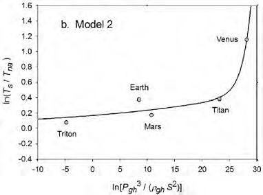

 Citation:
 N kolov N, Zeller K (2017) New Insights on the Physical Nature of the Atmospheric Greenhouse Effect Deduced from an Empirical Planetary
Temperature Model. Environ Pollut Climate Change 1: 112.
Page 7 of 22
ACT 1982
INFORMATION
Figure 1: The rela ive atmospheric thermal enhancement (
T /T ) as a function of various dimensionless
forcing variables generated by DA using data on solar
s
r
irradiance, near-surface partial pressure/den ity of greenhouse gases, and total atmospheric pressure/density from Table 4. Panels
a through
f depict six regression
models suggested by DA with the underlying celestial bodies plotted in the background for reference. Each pair of horizontal graphs represents different reference
RELEASED UNDER THE
temperatures (
T ) defined as either
T = T ( eft) or
T = T (right).
r
r
e
r
na
which excludes Titan from the input dataset. This new curve had
R2 =
Equation (10a) implies that GMATs of rocky planets can be
1.0 and σ = 0.0009. Although the two regression equations yield similar
calculated as a product of two quantities: the planet’s average surface
est
results over most of the relevant pressure range, we chose the one without
temperature in the absence of an atmosphere (
T , K) and a non-
na
Titan as final for Model 12 based on the assumption that Earth’s GMAT
dimensional factor (
E ≥ 1.0) quantifying the relative thermal effect of
a
is likely known with a much greater accuracy than Titan’s mean annual
the atmosphere, i.e.
temperature. Taking an antilogarithm of the final regression equation,
which excludes Titan, yielded the following expression fo
OFFICIAL r Model 12:
T =
T E
(10b)
s
na a
0.150263
1.04193
T
P
where
Τ is obtained from the SAT model (Eq. 4a) and
E is a function
−
P
s
5
= exp 0.174205
+ 1.83121 × 10
(10a)
na
a
of total pressure (
P) given by:
na
T
P
P
r
r
0.150263
1.04193
The regression coefficients in Eq. (10a) are intentional y shown in
P
−
P
E
P =
×
(11)
a (
)
5
exp 0.174205
exp 1.83121 10
full precision to allow an accurate calculation of RATE (i.e. the
T /
P
P
r
r
s
T ratios) provided the strong non-linearity of the relationship and
na
to facilitate a successful replication of our results by other researchers.
Note that, as
P approaches 0 in Eq. (11),
E approaches the physical y
a
Figure 4 depicts Eq. (10a) as a dependence of RATE on the average
realistic limit of 1.0. Other physical aspects of this equation are
surface air pressure. Superimposed on this graph are the six planetary
discussed below.
bodies from Table 4 along with their uncertainty ranges.
For bodies with tangible atmospheres (such as Venus, Earth,
Environ Pollut Climate Change, an open access journal
Volume 1 • Issue 2 • 1000112
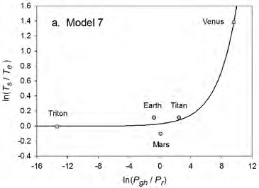


 Citation:
 N kolov N, Zeller K (2017) New Insights on the Physical Nature of the Atmospheric Greenhouse Effect Deduced from an Empirical Planetary
Temperature Model. Environ Pollut Climate Change 1: 112.
Page 8 of 22
ACT 1982
Figure 2: The same as in Figure 1 but for six additional regression models (panels
a through
f).
INFORMATION
Mars, Titan and Triton), one must calculate
T using
α = 0.132 and
surface in a way that transforms these parameters from independent
n
e
η = 0.00971, which assumes a Moon-like airless reference surface in
controllers of the global temperature in airless bodies to intrinsic
RELEASED UNDER THE
e
accordance with our pre-analysis premise For bodies with tenuous
byproducts of the climate system itself in worlds with appreciable
atmospheres (such as Mercury, he Moon, Calisto and Europa),
T na
atmospheres. In other words, once atmospheric pressure rises above a
should be calculated from Eq. (4a) (or Eq. 4b respectively if
S > 0.15
certain level, the effects of albedo and ground heat storage on GMAT
W m-2 and/or Rg ≈ 0 W m-2) using the body’s observed
values of Bond
become implicitly accounted for by Eq. (11). Although this hypothesis
albedo
α and ground heat storage fraction
η . In the context of this
e
e
requires a further investigation beyond the scope of the present study,
model, a tangible atmosphere is defined as one that has significantly
one finds an initial support for it in the observation that, according to
modified the optical and thermo-physical properties of a planet’s
data in Table 2, GMATs of bodies with tangible atmospheres do not
surface compared to an airless environment and/or noticeably show a physical y meaningful relationship with the amounts of absorbed
impacted the overall planetary albedo by enabling the formation of
shortwave radiation determined by albedos. Our discovery for the
OFFICIAL
clouds and haze. A tenuous atmosphere, on the other hand, is one that
has not had a measurable influence on the surface albedo and regolith
need to utilize different albedos and heat storage coefficients between
thermo-physical properties and is completely transparent to shortwave
airless worlds and worlds with tangible atmospheres is not unique as a
radiation. The need for such delineation of atmospheric masses when
methodological approach. In many areas of science and engineering,
calculating
T arises from the fact that Eq. (10a) accurately describes
it is sometime necessary to use disparate model parameterizations to
na
RATEs of planetary bodies with tangible atmospheres over a wide
successful y describe different aspects of the same phenomenon. An
range of conditions without explicitly accounting for the observed large
example is the distinction made in fluid mechanics between laminar
differences in albedos (i.e. from 0.235 to 0.90) while assuming constant
and turbulent flow, where the non-dimensional Reynold’s number is
values of
α and
η for the airless equivalent of these bodies. One possible
employed to separate the two regimes that are subjected to different
e
e
explanation for this counterintuitive empirical result is that atmospheric
mathematical treatments.
pressure alters the planetary albedo and heat storage properties of the
Environ Pollut Climate Change, an open access journal
Volume 1 • Issue 2 • 1000112

 Citation:
 N kolov N, Zeller K (2017) New Insights on the Physical Nature of the Atmospheric Greenhouse Effect Deduced from an Empirical Planetary
Temperature Model. Environ Pollut Climate Change 1: 112.
Page 9 of 22
No.
Functional Model
Coefficient of Determination (R2)
Adjusted R2
Standard Error σest
3
T
P
1
gh
s
=
f
2
0.9844
0.9375
0.1529
T
ρ
S
gh
e
3
T
P
2
gh
s
=
f
2
0.9562
0.8249
0.1773
T
ρ
S
gh
na
3
T
P
s
3
=
f
2
0.1372
-2.4511
1.1360
T
ρ
S
gh
e
3
T
P
s
4
=
f
2
0.2450
-2.0200
0.7365
T
ρ
S
gh
na
3
T
P
5
gh
s
=
f
2
0.9835
0.9339
0.1572
T
ρ
e
S
3
T
P
6
gh
s
=
f
2
0.9467
0.7866
0.1957
T
ρ
na
S
T
P
7
gh
s
=
f
0.9818
0.927
0.1648
e
T
P
r
T
P
8
gh
s
=
ACT 1982
f
0.9649
0.8598
0.1587
na
T
P
r
3
T
P
s
9
=
f
2
0.4488
-0.3780
0.7060
T
ρ
e
S
3
T
P
s
10
=
f
2
0.6256
0.0639
0.4049
T
ρ
na
S
T
P
11
s =
f
0.9396
0.8489
0.2338
e
T
P
r
T
P
12
s
=
f
0.9999
0.9997
0.0078
na
T
P
r
Table 5: Performance statistics of the twelve regression models suggested by DA. Statistical scores refer to the model logarithmic forms shown in Figures 1 and 2.
INFORMATION
RELEASED UNDER THE
OFFICIAL
Figure 3: Comparison of the two best-performing regression models according to statistical scores listed in Table 5. Vertical axes use linear scales to better illustrate
he difference in skills between the models.
We do not currently have sufficient data to precisely define the limit
and from Eq. (4a) (or Eq. 4b, respectively) using observed values of
α e
between
tangible and
tenuous atmospheres in terms of total pressure for
and
η if
P ≤ 10-2 Pa. Equation (4a) should also be employed in cases,
e
the purpose of this model. However, considering that an atmospheric
where a significant geothermal flux exists such as on the Galilean moons
pressure of 1.0 Pa on Pluto causes the formation of layered haze [93],
of Jupiter due to tidal heating, and/or if
S ≤ 0.15 W m-2. Hence, the
we surmise that this limit likely lies significantly below 1.0 Pa. In this
30-year mean global equilibrium surface temperature of rocky planets
study, we use 0.01 Pa as a tentative threshold value. Thus, in the context
depends in general on five factors: TOA stel ar irradiance (
S), a reference
of Eq. (10b), we recommend computing
T from Eq. (4c) if
P > 10-2 Pa,
na
airless surface albedo (
α ), a reference airless ground heat storage fraction
e
Environ Pollut Climate Change, an open access journal
Volume 1 • Issue 2 • 1000112

 Citation:
 N kolov N, Zeller K (2017) New Insights on the Physical Nature of the Atmospheric Greenhouse Effect Deduced from an Empirical Planetary
Temperature Model. Environ Pollut Climate Change 1: 112.
Page 10 of 22
K). Equation (10b) produces 95.18 K for Titan at Saturn’s semi-major
axis (9.582 AU) corresponding to a solar irradiance
S = 14.8 W m-2. This
estimate is virtual y identical to the 95 K average surface temperature
reported for that moon by the NASA JPL Voyager Mission website
[94]. The Voyager spacecraft 1 and 2 reached Saturn and its moons in
November 1980 and August 1981, respectively, when the gas giant was
at a distance between 9.52 AU and 9.60 AU from the Sun corresponding
approximately to Saturn’s semi-major axis [95].
Data acquired by Voyager 1 suggested an average surface
temperature of 94 ± 0.7 K for Titan, while Voyager 2 indicated a
temperature close to 95 K [41]. Measurements obtained between 2005
and 2010 by the Cassini-Huygens mission revealed
T ≈ 93.4 ± 0.6 K
s
[42,43]. Using Saturn’s perihelion (9.023 AU) and aphelion (10.05 AU)
one can compute Titan’s TOA solar irradiance at the closest and furthest
approach to the Sun, i.e 16 7 W m-2 and 13.47 W m-2, respectively.
Inserting these values into Eq. (10b) produces the expected upper and
Figure 4: The relative atmospheric thermal enhancement (
T /T ratio) as a
lower limit of Titan’s mean global surface temperature according to
s
na
function of the average surface air pressure according to Eq. (10a) derived from
our model, i.e. 92.9 K ≤
T ≤ 98.1 K. Notably this range encompasses
s
data representing a broad range of planetary environments in the solar system.
all current observation-based estimates of Titan’s GMAT. Since both
Saturn’s moon Titan has been excluded from the regression analysis leading
to Eq. (10a). Error bars of some bodies are not clearly visible due to their small
Voyager and C ssini mission covered shorter periods than a single
size relative to the scale of the axes. See Table 2 for the actual error estimates.
Titan eason (Saturn’s orbital period is 29.45 Earth years), the available
ACT 1982
measurements may not well represent that moon’s annual thermal
cycle. In addition due to a thermal inertia, Titan’s average surface
temperature likely lags variations in the TOA solar irradiance caused
by Saturn’s orbital eccentricity. Thus, the observed 1.45 K discrepancy
between our independent model prediction and Titan’s current
best-known GMAT seems to be within the range of plausible global
temperature fluctuations on that moon. Hence, further observations are
needed to more precisely constrain Titan’s long-term GMAT.
Measurements conducted by the Voyager spacecraft in 1989
indicated a global mean temperature of 38 ± 1.0 K and an average
atmospheric pressure of 1.4 Pa at the surface of Triton [73]. Even
though Eq. (10a) is based on slightly different data for Triton (i.e.
T =
s
39 ±1.0 K and
P = 4.0 Pa) obtained by more recent stel ar occultation
measurements [73], employing the Voyager-reported pressure in Eq.
(10b) produces
T = 38.5 K for Triton’s GMAT, a value well within the
s
uncertainty of the 1989 temperature measurements.
INFORMATION
The above comparisons indicate that Eq. (10b) rather accurately
Figure 5: Absolute differences b tween modeled average global temperatures
describes the observed variation of the mean surface temperature across
by Eq. (10b) and observed GMATs (Table 2) for he studied celestial bodies.
a wide range of planetary environments in terms of solar irradiance
RELEASED UNDER THE
Saturn’s moon Titan represents an independent data point, since it was excluded
from the regression analysis leading to Eq. (10a).
(from 1.5 W m-2 to 2,602 W m-2), total atmospheric pressure (from
near vacuum to 9,300 kPa) and greenhouse-gas concentrations (from
0.0% to over 96% per volume). While true that Eq. (10a) is based on
(
η ), the average geothermal flux reaching the surface (
R ), and the total
e
g
data from only 6 celestial objects, one should keep in mind that these
surface atmospheric pressure (
P). For planets with tangible atmospheres
constitute virtual y all bodies in the Solar System meeting our criteria
(
P > 10-2 Pa) and a negligible geothermal heating of the surface (
R ≈ 0),
g
for availability and quality of measured data. Although function (5)
the equilibrium GMAT becomes only a function of two factors:
S and
has 4 free parameters estimated from just 5-6 data points, there are no
P, i.e.
Τ = 32.44
S0.25
E (
P). The final model (Eq. 10b) can also be cast
s
α
signs of model overfitting in this case because (
a) Eq. (5) represents
in terms of
T as a function of a planet’s distance to the Sun (
r , AU) by
a monotonic function of a rigid shape that can only describe well
OFFICIAL
s
au
replacing
S in Equations (4a), (4b) or (4c) with 1360.9
r -2.
certain exponential pattern as evident from Figures 1 and 2 and the
au
Environmental scope and numerical accuracy of the new statistical scores in Table 5; (
b) a simple scatter plot of ln (
P/P ) vs. ln(
T /
r
s
T ) visibly reveals the presence of an exponential relationship free of
model
na
data noise; and (
c) no polynomial can fit the data points in Figure 2f
Figure 5 portrays the residuals between modeled and observed
as accurately as Eq. (5) while also producing a physical y meaningful
absolute planetary temperatures. For celestial bodies participating in
response curve similar to known pressure-temperature relationships in
the regression analysis (i.e. Venus, Earth, Moon, Mars and Triton), the
other systems. These facts indicate that Eq. (5) is not too complicated
maximum model error does not exceed 0.17 K and is well within the
to cause an over-fitting but just right for describing the data at hand.
uncertainty of observations. The error for Titan, an independent data
The fact that only one of the investigated twelve non-linear
point, is 1.45 K or 1.5% of that moon’s current best-known GMAT (93.7
regressions yielded a tight relationship suggests that Model 12 describes
Environ Pollut Climate Change, an open access journal
Volume 1 • Issue 2 • 1000112
 Citation:
 N kolov N, Zeller K (2017) New Insights on the Physical Nature of the Atmospheric Greenhouse Effect Deduced from an Empirical Planetary
Temperature Model. Environ Pollut Climate Change 1: 112.
Page 11 of 22
a macro-level thermodynamic property of planetary atmospheres
heretofore unbeknown to science. A function of such predictive power
spanning the entire breadth of the Solar System cannot be just a result
of chance. Indeed, complex natural systems consisting of myriad
interacting agents have been known to sometime exhibit emergent
responses at higher levels of hierarchical organization that are amenable
to accurate modeling using top-down statistical approaches [96].
Equation (10a) also displays several other characteristics discussed
below that lend further support to the above notion.
Model robustness
Model robustness defines the degree to which a statistical
relationship would hold when recalculated using a different dataset. To
test the robustness of Eq. (10a) we performed an alternative regression
analysis, which excluded Earth and Titan from the input data and
only utilized logarithmic pairs of
T /T and
P/P for Venus, the Moon,
s
na
r
Mars and Triton from Table 4. The goal was to evaluate how well the
Figure 6: Demonstration of
the robustness f Model 12. The solid black curve
resulting new regression equation would predict the observed mean
depicts Eq. (10a) based on data from 5 celestial bodies (i.e. Venus, Earth, Moon,
surface temperatures of Earth and Titan. Since these two bodies occupy
Mars and Triton). The dashed grey curve portrays Eq. (12a) derived from data of
a highly non-linear region in Model 12 (Figure 2f), eliminating them
only 4 bodies (i e. Venus, Moon Mars and Triton) while excluding Earth and Titan
from the r gre sion analysis. The alternative Eq. (12b) predicts the observed
from the regression analysis would leave a key portion of the curve
GMATs of Ea th and Titan with accuracy greater han 99% indicating that Model
ACT 1982
poorly defined. As in all previous cases, function (5) was fitted to the
12 is statistically robust.
incomplete dataset (omitting Earth and Titan), which yielded the
following expression:
The above characteristics of Eq. (10a) including dimensional
0.150275
3.32375
T
P
homogeneity high predictive accuracy, broad environmental scope of
−
P
s
15
= exp 0.174222
+ 5.25043×10
(12 )
validity and sta istical robustness indicate that it represents an emergent
na
T
P
P
r
r
macro-physical model of theoretical significance deserving further
Substituting the reference temperature
T in Eq. (12a) with its investigation. This conclusive result is also supported by the physical
na
equivalent from Eq. (4c) and solving for
T produces
meaningfulness of the response curve described by Eq. (10a).
s
0.150275
3.32375
Discussion
0.25
P
15
−
P
(12b)
T =
S
×
s
32 44
exp 0 174222
exp 5 25043 10
P
P
r
r
Given the high statistical scores of the new model discussed above,
It is evident that the regression coefficients in the first exponent term of
it is important to address its physical significance, potential limitations,
Eq. (12a) are nearly identical to those in Eq. (10a). This term dominates
and broad implications for the current climate theory.
the
T -P relationship over the pressure range 0-400 kPa ccounting
s
Similarity of the new model to Poisson’s formula and the SB
for more than 97.5% of the predicted temperature magnitudes. The
regression coefficients of the second exponent differ somewhat between
radiation law
the two formulas causing a diverg nce of calculated RATE values
The functional response of E
INFORMATION q. (10a) portrayed in Figure 4 closely
over the pressure interval 400–9,100 kPa. Th models converge again
resembles the shape of the dry adiabatic temperature curve in Figure
between 9,000 kPa and 9,300 kPa. Figure 6 il ustrates the similarity of
7a described by the Poisson formula and derived from the First Law of
RELEASED UNDER THE
responses between Equations (10a) and (12a) over the pressure range
Thermodynamics and the Ideal Gas Law [4], i.e.
0–300 kPa with Earth and Titan plotted in the foreground for reference.
R/
cp
T
p
=
(13)
Equation (12b) reproduces the observed global surface temperature
T
p
o
o
of Earth with an error of 0 4% (-1.0 K) and that of Titan with an error
of 1.0% (+0.9 K). For Titan, the error of the new Eq. (12b) is even
Here,
T and
p are reference values for temperature and pressure
o
o
slightly smaller than that of the original model (Eq. 10b). The ability
typical y measured at the surface, while
T and
p are corresponding scalars
of Model 12 to predict Earth’s GMAT with an accuracy of 99.6% using
in the free atmosphere, and
c is the molar heat capacity of air (J mol-1
p
a relationship inferred from disparate environments such as those
K-1). For the Earth’s atmosphere,
R/c = 0.286. Equation (13) essential y
p
found on Venus, Moon, Mars and Triton indicates tha
OFFICIAL t (
a) this model describes the direct effect of pressure
p on the gas temperature (
T) in
is statistical y robust, and (
b) Earth’s temperature is a part of a cosmic
the absence of any heat exchange with the surrounding environment.
thermodynamic continuum well described by Eq. (10b). The apparent
Equation (10a) is structural y similar to Eq. (13) in a sense that
smoothness of this continuum for bodies with tangible atmospheres
both expressions relate a temperature ratio to a pressure ratio, or more
(il ustrated in Figure 4) suggests that planetary climates are well-
precisely, a relative thermal enhancement to a ratio of physical forces.
buffered and have no ‘tipping points’ in reality, i.e. states enabling
However, while the Poisson formula typical y produces 0 ≤
T/T ≤ 1.0,
o
rapid and irreversible changes in the global equilibrium temperature
Eq. (10a) always yields
T /T ≥ 1.0. The key difference between the two
s
na
as a result of destabilizing positive feedbacks assumed to operate within
models stems from the fact that Eq. (13) describes vertical temperature
climate systems. This robustness test also serves as a cross-validation
changes in a free and
dry atmosphere induced by a gravity-controlled
suggesting that the new model has a universal nature and it is not a
pressure gradient, while Eq. (10a) predicts the equilibrium response of a
product of overfitting.
planet’s global surface air temperature to variations in total atmospheric
Environ Pollut Climate Change, an open access journal
Volume 1 • Issue 2 • 1000112

 Citation:
 N kolov N, Zeller K (2017) New Insights on the Physical Nature of the Atmospheric Greenhouse Effect Deduced from an Empirical Planetary
Temperature Model. Environ Pollut Climate Change 1: 112.
Page 12 of 22
Figure 7: Known pressure-temperature kinetic relations: (
a)
Dry adiabatic response of the air/surface temperature ratio to pressure changes in a free dry atmosphere
according to Poisson’s formula (Eq. 13) with a reference pressure set to
p = 100 kPa; (
b) The SB radiation law expressed as a response of a blackbody temperature
o
ratio to variations in photon pressure (Eq. 14). Note he qualitative striking similarity of shapes between these curves and the one portrayed in Figure 4 depicting the
new planetary temperature model (Eq. 10a).
pressure. In essence, Eq. (10b) could be viewed as a predictor of the
boosts the int rnal kinetic energy and raises its temperature, a process
reference temperature
T in the Poisson formula. Thus, while qualitatively
known in thermodynamics as compression heating. The direct effect
o
similar, Equations (10a) and (13) are quantitatively rather different. Both
of pressure on a system’s temperature is thermodynamical y described
ACT 1982
functions describe effects of pressure on temperature but in the context of
by adi batic proce ses The pressure-induced thermal enhancement
disparate physical systems. Therefore, estimates obtained from Eq. (10a)
at a planetary lev l portrayed in Figure 4 and accurately quantified by
should not be confused with results inferred from the Poisson formula.
Eq (10a or 11) is analogous to a compression heating, but not ful y
For example, Eq. (10b) cannot be expected to predict the temperature
i entical to an adiabatic process. The latter is usual y characterized by
lapse rate and/or vertical temperature profiles within a planetary a limited duration and oftentimes only applies to finite-size parcels of
atmosphere as could be using Eq. (13). Furthermore, Eq. (10a) represents
air moving vertical y through the atmosphere. Equation (11), on the
a top-down empirical model that implicitly accounts for a plethora of
other hand, describes a surface thermal effect that is global in scope and
thermodynamic and radiative processes and feedbacks operating in real
permanent in nature as long as an atmospheric mass is present within
climate systems, while the Poisson formula (derived from the Ideal Gas
the planet’s gravitational field. Hence, the planetary RATE (
T /T ratio)
s
na
Law) only describes pressure-induced temperature changes in a simple
c uld be understood as a net result of countless simultaneous adiabatic
mixture of dry gases without any implicit or explicit consideration of
processes continuously operating in the free atmosphere. Figures 4 and
planetary-scale mechanisms such as latent heat transport and cloud
7 also suggest that the pressure control of temperature is a universal
radiative forcing.
thermodynamic principle applicable to systems ranging in complexity
Equation (10a) also shows a remarkable similarity o the SB law
from a simple isothermal blackbody absorbing a homogeneous flux of
relating the equilibrium skin temp rature f an isotherma blackbody
electromagnetic radiation to diverse planetary atmospheres governed
(
T , K) to the electromagnetic radiati e flux (
I, W m
by complex non-linear process interactions and cloud-radiative
-2) absorbed/
b
INFORMATION
emitted by the body’s surface, i .
T = (
I ⁄ σ)
feedbacks. To our knowledge, this cross-scale similarity among various
0.25. Dividing each side of
this fundamental relationship by the irreducible temperature of deep
pressure-temperature relationships has not previously been identified
Space
T = 2.725 K and its causative CMBR
R = 3.13 × 10
and could provide a valuable new perspective on the working of
-6 W m-2
c
c
RELEASED UNDER THE
respectively, yields
T ⁄T = (
I ⁄
R )
planetary climates.
0.25. Further, expressing the radiative
b c
c
fluxes
I and
R on the right-hand side as products of photon pressure
Nevertheless, important differences exist between Eq. (10a) and
c
and the speed of light (
c, m s-1) in a vacuum, i.e.
I = cP and
R = cP ,
these other
simpler pressure-temperature relations. Thus, while the
ph
c
c
leads to the following alternative f rm of the SB law:
Poisson formula and the SB radiation law can mathematical y be
0 25
derived from ‘first principles’ and experimental y tested in a laboratory,
T
P
ph
b =
(14)
Eq. (10a) could neither be analytical y
deduced from known physical
T
P
c
c
laws nor accurately simulated in a small-scale experiment. This is
where
P = 1.043 × 10⁻¹⁴ Pa is the photon pressure of CMBR. Clearly, Eq.
c
because Eq. (10a) describes an emergent
macro-level property of
(10a) is analogous to Eq. (14), while the latter is structural y identical to
planetary atmospheres representing the net result of myriad process
the Poisson formula (13). Figure 7b depicts Eq. (14) as a dep
OFFICIAL endence of interactions within real climate systems that are not readily computable
the
T /
T ratio on photon pressure
P .
b
c
ph
using mechanistic (bottom-up) approaches adopted in climate models
It is evident from Figures 4 and 7 that formulas (10a), (13) and (14)
or ful y reproducible in a laboratory setting.
describe qualitatively very similar responses in quantitatively vastly
Potential limitations of the planetary temperature model
different systems. The presence of such similar relations in otherwise
disparate physical systems can fundamental y be explained by the fact
Equation (10b) describes long-term (30-year) equilibrium GMATs
that pressure as a force per unit area represents a key component of
of planetary bodies and does not predict inter-annual global temperature
the internal kinetic energy (defined as a product of gas volume and
variations caused by intrinsic fluctuations of cloud albedo and/or ocean
pressure), while temperature is merely a physical manifestation of this
heat uptake. Thus, the observed 0.82 K rise of Earth’s global temperature
energy. Adding a force such as gas pressure to a physical system inevitably
since 1880 is not captured by our model, as this warming was likely
Environ Pollut Climate Change, an open access journal
Volume 1 • Issue 2 • 1000112
Citation: N kolov N, Zeller K (2017) New Insights on the Physical Nature of the Atmospheric Greenhouse Effect Deduced from an Empirical Planetary
Temperature Model. Environ Pollut Climate Change 1: 112.
Page 13 of 22
not the result of an increased atmospheric pressure. Recent analyses of
significantly over the past 65.5 My could open exciting new research
observed dimming and brightening periods worldwide [97-99] suggest
venues in Earth sciences in general and paleoclimatology in particular.
that the warming over the past 130 years might have been caused by a
decrease in global cloud cover and a subsequent increased absorption of
Role of greenhouse gasses from a perspective of the new
solar radiation by the surface. Similarly, the mega shift of Earth’s climate
model
from a ‘hothouse’ to an ‘icehouse’ evident in the sedimentary archives
Our analysis revealed a poor relationship between GMAT and the
over the past 51 My cannot be explained by Eq. (10b) unless caused by
amount of greenhouse gases in planetary atmospheres across a broad
a large loss of atmospheric mass and a corresponding significant drop
range of environments in the Solar System (Figures 1-3 and Table 5).
in surface air pressure since the early Eocene. Pleistocene fluctuations
This is a surprising result from the standpoint of the current Greenhouse
of global temperature in the order of 3.0–8.0 K during the last 2 My
theory, which assumes that an atmosphere warms the surface of a planet
revealed by multiple proxies [100] are also not predictable by Eq. (10b)
(or moon) via trapping of radiant heat by certain gases controlling the
if due to factors other than changes in total atmospheric pressure and/
atmospheric infrared optical depth [4,9,10]. The atmospheric opacity
or TOA solar irradiance.
to LW radiation depends on air density and gas absorptivity, which in
The current prevailing view mostly based on theoretical turn are functions of total pressure, temperature and greenhouse-gas
considerations and results from climate models is that the Pleistocene
concentrations [9]. Pressure also controls the broadening of infrared
glacial-interglacial cycles have been caused by a combination of three
absorption lines in individual gases. Therefore, the higher the pressure,
forcing agents: Milankovitch orbital variations, changes in atmospheric
the larger the infrared optical depth of an atmosphere, and the stronger
the expected greenhouse effect would be. According to the current
concentrations of greenhouse gases, and a hypothesized positive ice-
climate theory, pressure only indirectly affects global surface temperature
albedo feedback [101,102]. However, recent studies have shown that
through the atmospheric infrared opacity and its presumed constraint on
orbital forcing and the ice-albedo feedback cannot explain key features
the planet’s LW emission to Space [9,107].
of the glacial-interglacial oscil ations such as the observed magnitudes
ACT 1982
of global temperature changes, the skewness of temperature response
There are four plausible explanations for the apparent lack of a
(i.e. slow glaciations followed by rapid meltdowns), and the mid-
close relationship between GMAT and atmospheric greenhouse gasses
Pleistocene transition from a 41 Ky to 100 Ky cycle length [103-105]. The
in ur results: 1) The amounts of greenhouse gases considered in our
only significant forcing remaining in the present paleo-climatological
analysis only refer to near-surface atmospheric compositions and
toolbox to explicate the Pleistocene cycles are variations in greenhouse-
do not de cribe the infrared optical depth of the entire atmospheric
gas concentrations. Hence, it is difficult to explain, from a standpoint
column; 2) The analysis lumped all greenhouse gases together and did
of the current climate theory, the high accuracy of Eq. (11) describing
not take into account differences in the infrared spectral absorptivity of
the relative thermal effect of diverse planetary atmospheres without any
individual gasses; 3) The effect of atmospheric pressure on broadening
consideration of greenhouse gases. If presumed forcing agents such as
the infrared gas absorption lines might be stronger in reality than
greenhouse-gas concentrations and the planetary albedo were ind ed
simulated by current radiative-transfer models, so that total pressure
responsible for the observed past temperature dynamics on Earth, why
overrides the effect of a varying atmospheric composition across a wide
did these agents not show up as predictors of contemporary planetary
range of planetary environments; and 4) Pressure as a force per unit area
temperatures in our analysis as well? Could it be because the e agents
directly impacts the internal kinetic energy and temperature of a system
have not real y been driving Earth’s climate on geological time scales?
in accordance with thermodynamic principles inferred from the Gas
We address the potential role of greenhouse gases in more d tails below.
Law; hence, air pressure might be the actual physical causative factor
Since the relationship portrayed in Figure 4 is undoubtedly real, our
controlling a planet’s surface temperature rather than the atmospheric
INFORMATION
model results point toward the need to reexamine some fundamental
infrared optical depth, which merely correlates with temperature due to
climate processes thought to be well understood for decades. For
its co-dependence on pressure.
example, we are currently testing a hypo hesi that Pleistocene glacial
Based on evidence discussed earlier, we argue that option #4 is
RELEASED UNDER THE
cycles might have been caused by variations in Earth’s total atmospheric
the most likely reason for the poor predictive skill of greenhouse
mass and surface air pressure. Preliminary results based on the ability
gases with respect to planetary GMATs revealed in our study (Figures
of an extended version of our planetary model (simulating meridional
1-3). By definition, the infrared optical depth of an atmosphere is a
temperature gradients) to predict the observed polar amplification
dimensionless quantity that carries no units of force or energy [3,4,9].
during the Last Glacial Maximum indicate that such a hypothesis is not
Therefore, it is difficult to fathom from a fundamental physics standpoint
unreasonable. However conclusive findings from this research will be
of view, how this non-dimensional parameter could increase the kinetic
discussed elsewhere.
energy (and temperature) of the lower troposphere in the presence of
free convection provided that the latter dominates the heat transport in
According to the present understanding, Earth’s atmospheric gaseous systems. Pressure, on the other hand, has a dimension of force
pressure has remained nearly invariant during the Cen
OFFICIAL ozoic era (last per unit area and as such is intimately related to the internal kinetic
65.5 My). However, this notion is primarily based on theoretical
energy of an atmosphere
E (J) defined as the product of gas pressure (
P,
analyses [106], since there are currently no known geo-chemical proxies
Pa) and gas volume (
V, m3), i.e.
E (J) =
PV. Hence, the direct effect of
permitting a reliable reconstruction of past pressure changes in a
pressure on a system’s internal energy and temperature follows straight
manner similar to that provided by various temperature proxies such as
from fundamental parameter definitions in classical thermodynamics.
isotopic oxygen 18, alkenones and TEX in sediments, and Ar-N isotope
86
General y speaking, kinetic energy cannot exist without a pressure
ratios and deuterium concentrations in ice. The lack of independent
force. Even electromagnetic radiation has pressure.
pressure proxies makes the assumption of a constant atmospheric mass
throughout the Cenozoic
a priori and thus questionable. Although
In climate models, the effect of infrared optical depth on surface
this topic is beyond the scope of our present study, allowing for the
temperature is simulated by mathematical y decoupling radiative
possibility that atmospheric pressure on Earth might have varied
transfer from convective heat exchange. Specifical y, the LW
Environ Pollut Climate Change, an open access journal
Volume 1 • Issue 2 • 1000112
Citation: N kolov N, Zeller K (2017) New Insights on the Physical Nature of the Atmospheric Greenhouse Effect Deduced from an Empirical Planetary
Temperature Model. Environ Pollut Climate Change 1: 112.
Page 14 of 22
radiative transfer is calculated in these models without simultaneous
is fundamental y different from the hypothesized ‘trapping’ of LW
consideration of sensible- and latent heat fluxes in the solution matrix.
radiation by atmospheric trace gases first proposed in the 19th century
Radiative transfer modules compute the so-called heating rates (K/
and presently forming the core of the Greenhouse climate theory.
day) strictly as a function of atmospheric infrared opacity, which
However, a radiant-heat trapping by freely convective gases has never
under constant-pressure conditions solely depends on greenhouse-
been demonstrated experimental y. We should point out that the hereto
gas concentrations. These heating rates are subsequently added to the
deduced adiabatic (pressure-controlled) nature of the atmospheric
thermodynamic portion of climate models and distributed throughout
thermal effect rests on an objective analysis of vetted planetary
the atmosphere. In this manner, the surface warming becomes a
observations from across the Solar System and is backed by proven
function of an increasing atmospheric infrared opacity. This approach to
thermodynamic principles, while the ‘trapping’ of LW radiation by an
modeling of radiative-convective energy transport rests on the principle
unconstrained atmosphere surmised by Fourier, Tyndall and Arrhenius
of superposition, which is only applicable to linear systems, where the
in the 1800s was based on a theoretical conjecture. The la ter has later
overall solution can be obtained as a sum of the solutions to individual
been coded into algorithms that describe the surface temperature as a
system components. However, the integral heat transport within a
function of atmospheric infrared optical depth (instead of pressure) by
free atmosphere is inherently nonlinear with respect to temperature.
artificial y decoupling radiative transfer from convective heat exchange.
This is because, in the energy balance equation, radiant heat transfer
Note also that the Ideal Gas Law (
PV = nRT) forming the basis of
is contingent upon power gradients of absolute temperatures, while
atmospheric physics is indifferent to the gas chemical composition.
convective cooling/heating depends on linear temperature differences
Effect of pressure on temperature: Atmospheric pressure
in the case of sensible heat flux and on simple vapor pressure gradients
provides in and of i self only a elative thermal enhancement (RATE)
in the case of latent heat flux [4]. The latent heat transport is in turn
to the surface quantified by Eq. (11). The absolute thermal effect of an
a function of a solvent’s saturation vapor pressure, which increases
atmosphere depends on both pressure and the TOA solar irradiance.
exponential y with temperature [3]. Thus, the superposition principle
For example, at a total air pressure of 98.55 kPa, Earth’s RATE is 1.459,
ACT 1982
cannot be employed in energy budget calculations. The artificial which keeps our planet 90 4 K warmer in its present orbit than it would
decoupling between radiative and convective heat-transfer processes
be in the absence of n atmosphere. Hence, our model ful y explains
adopted in climate models leads to mathematical y and physical y
the new ~90 K estimate of Earth’s atmospheric thermal effect derived
incorrect solutions with respect to surface temperature. The LW by Volokin and ReLlez [1] using a different line of reasoning. If one
radiative transfer in a real climate system is intimately intertwined
moves Earth to the orbit of Titan (located at ~9.6 AU from the Sun)
with turbulent convection/advection as both transport mechanisms
without changing the overall pressure, our planet’s RATE will remain
occur simultaneously. Since convection (and especial y the moist one)
the same, but the absolute thermal effect of the atmosphere would drop
is orders of magnitude more efficient in transferring energy than LW
to about 29.2 K due to a vastly reduced solar flux. In other words, the
radiation [3,4], and because heat preferential y travel along the path
absolute effect of pressure on a system’s temperature depends on the
of least resistance, a properly coupled radiative-conv ctive algorithm
background energy level of the environment. This implies that the
of energy exchange will produce quantitatively and qualitatively absolute temperature of a gas may not follow variations of pressure
different temperature solutions in response to a changing atmospheric
if the gas energy absorption changes in opposite direction to that of
composition than the ones obtained by current climate models. pressure. For instance, the temperature of Earth’s stratosphere increases
Specifical y, a correctly coupled convective-radiative system will render
with altitude above the tropopause despite a falling air pressure, because
the surface temperature insensitive to v riations in the atmospheric
the absorption of UV radiation by ozone steeply increases with height,
infrared optical depth, a result indir ctly supported by our analysis as
thus offsetting the effect of a dropping pressure. If the UV absorption
wel . This topic requires furth r investigation beyond the scope of the
were constant throughout the stratosphere, the air temperature would
INFORMATION
present study.
decrease with altitude.
The direct effect of atmospheric pressure on the global surface
Atmospheric back radiation and surface temperature: Since
RELEASED UNDER THE
temperature has received virtual y no a tention in climate science thus
(according to Eq. 10b) the equilibrium GMAT of a planet is mainly
far. However, the results from our empirical data analysis suggest that it
determined by the TOA solar irradiance and surface atmospheric
deserves a serious consideration in the future.
pressure, the down-welling LW radiation appears to be global y a product
of the air temperature rather than a driver of the surface warming. In
Theoretical implications of the new interplanetary other words, on a planetary scale, the so-called back radiation is a
relationship
consequence of the atmospheric thermal effect rather than a cause for
The hereto discovered pressure-temperature relationship quantified
it. This explains the broad variation in the size of the observed down-
by Eq. (10a) and depicted in Figure 4 has broad theoretical implications
welling LW flux among celestial bodies irrespective of the amount of
that can be summarized as follows:
absorbed solar radiation. Therefore, a change in this thermal flux brought
OFFICIAL
about by a shift in atmospheric LW emissivity cannot be expected to
Physical nature of the atmospheric ‘greenhouse effect’: According
impact the global surface temperature. Any variation in the global
to Eq. (10b), the heating mechanism of planetary atmospheres is
infrared back radiation caused by a change in atmospheric composition
analogous to a gravity-controlled adiabatic compression acting upon
would be compensated for by a corresponding shift in the intensity of
the entire surface. This means that the atmosphere does not function
the vertical convective heat transport. Such a balance between changes
as an insulator reducing the rate of planet’s infrared cooling to space as
in atmospheric infrared heating and the upward convective cooling at
presently assumed [9,10], but instead adiabatical y boosts the kinetic
the surface is required by the First Law of Thermodynamics. However,
energy of the lower troposphere beyond the level of solar input through
current climate models do not simulate this compensatory effect of
gas compression. Hence, the physical nature of the atmospheric sensible and latent heat fluxes due to an improper decoupling between
‘greenhouse effect’ is a pressure-induced thermal enhancement radiative transfer and turbulent convection in the computation of total
(PTE) independent of atmospheric composition. This mechanism energy exchange.
Environ Pollut Climate Change, an open access journal
Volume 1 • Issue 2 • 1000112
Citation: N kolov N, Zeller K (2017) New Insights on the Physical Nature of the Atmospheric Greenhouse Effect Deduced from an Empirical Planetary
Temperature Model. Environ Pollut Climate Change 1: 112.
Page 15 of 22
Role of planetary albedos: The fact that Eq. (10b) accurately
atmospheric pressure and an extremely cold environment found on that
describes planetary GMATs without explicitly accounting for the moon. Thus, our analysis did not reveal evidence for the existence of a
observed broad range of albedos, i.e. from 0.136 to 0.9 (Table 2),
feedback between planetary GMAT and a precipitable liquid solvent on
indicates that the shortwave reflectivity of planetary atmospheres is
the surface as predicted by the current climate theory. Consequently,
mostly an intrinsic property (a byproduct) of the climate system itself
the hypothesized
runaway greenhouse, which requires a net positive
rather than an independent driver of climate as currently believed. In
feedback between global surface temperature and the atmospheric LW
other words, it is the internal energy of the atmosphere maintained by
opacity controlled by water vapor [117], appears to be a model artifact
solar irradiance and air pressure that controls the bulk of the albedo.
rather than an actual physical possibility. Indeed, as il ustrated in Figure
An indirect support for this unorthodox conclusion is provided by
4, the hot temperature of Venus often cited as a product of a ‘runaway
the observation that the amounts of absorbed shortwave radiation
greenhouse’ scenario [117,118] fits perfectly within the pressure-
determined by albedos show no physical y meaningful relationship
dependent climate continuum described by Equations (10 ) and (11).
with planetary GMATs. For example, data in Table 2 indicate that
Venus absorbs 3.7 times less solar energy per unit area than Earth, yet
Model Application and Validation
its surface is about 450 K hotter than that of Earth; the Moon receives
Encouraged by the high predictive skill and broad scope of validity
on average 54 W m-2 more net solar radiation than Earth, but it is
of Model 12 (Figure 2f) we decided to apply Eq. (10b) to four celestial
about 90 K cooler on average than our planet. The hereto proposed
bodies spanning the bread h of the Solar System, i.e. Mercury, Europa,
passive nature of planetary albedos does not imply that the global
Callisto and Pluto which global surface temperatures are not currently
cloud cover could not be influenced by an external forcing such as solar
known with certainty. Each body is the target of either ongoing or
wind, galactic cosmic rays, and/or gravitational fields of other celestial
planned robotic exploration missions scheduled to provide surface
objects. Empirical evidence strongly suggests that it can [108-113], but
thermal d ta among other observations, thus offering an opportunity
the magnitude of such influences is expected to be small compared to
to validate our planetary temperature model against independent
ACT 1982
the total albedo due to the presence of stabilizing negative feedbacks
measurements.
within the system. We also anticipate that the sensitivity of GMATs to
an albedo change will greatly vary among planetary bodies. Viewing
The MESSENGER spacecraft launched in 2004 completed the first
the atmospheric reflectivity as a byproduct of the available internal
comprehensive mapping of Mercury in March 2013 (http://messenger.
energy rather than a driver of climate can also help explain the observed
jhuapl.edu/). Among other things, the spacecraft also took infrared
remarkable stability of Earth’s albedo [54,114].
measurements of the planet’s surface using a special spectrometer
Climate stability: Our semi-empirical model (Equations 4a, 10b
[119] th t should soon become available. The New Horizons spacecraft
and 11) suggests that, as long as the mean annual TOA solar flux and
launched in January 2006 [120] reached Pluto in July of 2015 and
the total atmospheric mass of a planet are stationary, the eq ilibrium
performed a thermal scan of the dwarf planet during a flyby. The
GMAT will remain stable. Inter-annual and decadal variations of global
complete dataset from this flyby were received on Earth in October of
temperature forced by fluctuations of cloud cove , for exampl , ar
2016 and are currently being analyzed. A proposed joint Europa-Jupiter
expected to be small compared to the magnitude of the background
System Mission by NASA and the European Space Agency is planned to
atmospheric warming because of strong neg tive feedbacks limiting
study the Jovian moons after year 2020. It envisions exploring Europa’s
the albedo changes. This implies a rela ively stable clim te for a planet
physical and thermal environments both remotely via a NASA Orbiter
such as Earth absent significant shifts in the total tmospheric mass
and
in situ by a Europa Lander [121].
and the planet’s orbital distance to the Sun. Hence, planetary climates
All four celestial bodies have somewhat eccentric orbits around the
appear to be free of tipping points, i.e. functional states fostering
INFORMATION
Sun. However, while Mercury’s orbital period is only 88 Earth days,
rapid and irreversible change in the global temperature as a result of
Europa and Callisto circumnavigate the Sun once every 11.9 Earth
hypothesized positive feedbacks thought to operate within the system.
years while Pluto takes 248 Earth years. The atmospheric pressure on
RELEASED UNDER THE
In other words, our results suggest that the Earth’s climate is well
Pluto is believed to vary between 1.0 and 4.0 Pa over the course of its
buffered against sudden changes.
orbital period as a function of insolation-driven sublimation of nitrogen
Effect of oceans and water vapor on global temperature: The new
and methane ices on the surface [122]. Each body’s temperature was
model shows that the Earth’s global equilibrium temperature is a part
evaluated at three orbital distances from the Sun: aphelion, perihelion,
of a cosmic thermodynamic continuum controlled by atmospheric
and the semi-major axis. Since Mercury, Europa and Callisto harbor
pressure and total solar irradiance. Since our planet is the only one
tenuous atmospheres (
P << 10-2 Pa), the reference temperature
T in
na
among studied celesti l bodies harboring a large quantity of liquid
Eq. (10b) must be calculated from Eq. (4a), which requires knowledge
water on the surface, Eq. (10b) implies that the oceans play virtual y no
of the actual values of
α ,
η , and
R . We assumed that Mercury had
R =
role in determining Earth’s GMAT. This finding may sound inexplicable
e
e
g
g
0.0 W m-2,
α = 0.068 [123] and Moon-like thermo-physical properties
OFFICIAL
from the standpoint of the radiative Greenhouse theory, but it follows
e
of the regolith (
η = 0.00971). Input data for Europa and Callisto were
logical y from the new paradigm of a pressure-induced atmospheric
e
obtained from Spencer et al. [124] and Moore et al. [125], respectively.
warming. The presence of liquid water on the surface of a planet requires
Specifical y, in order to calculate
η and
R for these moons we utilized
an air pressure greater than 612 Pa and an ambient temperature above
e
g
equatorial temperature data provided by Spencer et al. [124] in their
273.2 K. These conditions are provided by the planet’s size and gravity,
Figure 1, and by Moore et al. [125] in their Fig. 17.7 along with a
its distance to the Sun, and the mass of the atmosphere. Hence, the
theoretical formula for computing the average nighttime surface
water oceans on Earth seem to be a thermodynamic consequence of
temperature
T at the equator based on the SB law, i.e.
particular physical conditions set by cosmic arrangements rather than
an active controller of the global climate. Similarly, the hydrocarbon
S ( −α )
0.25
1
η +
R
e
g
T =
lakes on the surface of Titan [115,116] are the result of a high
0.98 σ
(15)
Environ Pollut Climate Change, an open access journal
Volume 1 • Issue 2 • 1000112
Citation: N kolov N, Zeller K (2017) New Insights on the Physical Nature of the Atmospheric Greenhouse Effect Deduced from an Empirical Planetary
Temperature Model. Environ Pollut Climate Change 1: 112.
Page 16 of 22
where
S(1-
α)
η is the absorbed solar flux (W m-2) stored as heat into
wel be within the uncertainty of Pluto’s true global temperature. We
e
the subsurface. The geothermal heat flux on Europa is poorly known.
will know more about this in 2017 when spatially resolved thermal
However, based on thermal observations of Io reported by Veeder et al.
measurements obtained by New Horizons become available.
[126], we assumed
R = 2.0 W m-2 for Europa. Using
S = 50.3 W m-2, an
g
observed nighttime equatorial temperature
T = 90.9 K and an observed
One should use caution when comparing results from Eq. (10b)
average night-side albedo
α = 0.58 [124], we solved Eq. (15) for the
to remotely sensed ‘average temperatures’ commonly quoted for
surface heat storage fraction to obtain
η = 0.085 for Europa. A similar
celestial bodies with tenuous atmospheres such as the moons of Jupiter
e
computational procedure was employed for Callisto using
α = 0.11 and
and Neptune. Studies oftentimes report the so-called ‘brightness
equatorial surface temperature data from Fig. 17.7 in Moore et al. [125].
temperatures’ retrieved at specific wavelengths that have not been
This produced
R = 0.5 W m-2 and
η = 0.057. Using these values in
subjected to a proper spherical integration. As pointed out by Volokin
g
e
Eq. (15) correctly reproduced Callisto’s nighttime equatorial surface
and ReLlez [1], due to Hölder’s inequality between integrals, calculated
temperature of ≈ 86.0 K. The much higher
η estimates for Europa and
brightness temperatures of spherical objects can be significantly higher
e
Callisto compared to
η = 0.00971 for the Moon can be explained with
than actual mean kinetic temperatures of the surface Sin e Eq. (10b)
e
the large water-ice content on the surface of these Galilean moons.
yields spherically averaged temperatures, its predictions for airless
Europa is almost completely covered by a thick layer of water ice, which
bodies are expected to be lower than the disk integrated brightness
has a much higher thermal conductivity than the dry regolith. Also,
temperatures typical y quoted in the literature.
sunlight penetrates deeper into ice than it does into powdered regolith.
Conclusion
All this enables a much larger fraction of the absorbed solar radiation to
be stored into the subsurface as heat and later released at night boosting
For 190 years the atmosphere has been thought to warm Earth
the nighttime surface temperatures of these moons. Volokin and ReLlez
by absorbing a portion of the outgoing LW infrared radiation and
[1] showed that GMAT of airless bodies is highly sensitive to
η .
reemitting it back toward the surface, thus augmenting the incident
e
solar flux This conceptualized continuous absorption and do
ACT 1982wnward
Table 6 lists the average global surface temperatures of the four
reemission of thermal radiation enabled by certain trace gases known
celestial bodies predicted by Eq. (10b) along with the employed input
to be transparent to solar rays while opaque to electromagnetic
data. According to our model, Mercury is about 117 K cooler on average
long wavelengths ha been likened to the trapping of heat by glass
than NASA’s current estimate of 440 K [32], which is based on Eq. (3)
greenhouses, hence the term ‘atmospheric greenhouse effect’. Of course,
and does not represent a spherically averaged surface temperature [1]
we now know that real greenhouses preserve warmth not by trapping
Our prediction of Europa’s GMAT, 99.4 K, agrees wel with the ≈ 100
infrared radiation but by physical y obstructing the convective heat
K estimate reported for this moon by Sotin et al. [127]. Our estimate
exchange between a greenhouse interior and the exterior environment.
of Pluto’s average surface temperature at perihelion (38.6 K) is similar
Nevertheless, the term ‘greenhouse effect’ stuck in science.
to the mean temperature computed for that dwarf planet by Olkin et
al. [124] using a mechanistic model of nitrogen ice volatilization at
The hypothesis that a freely convective atmosphere could retain
the surface. Stern et al. [128] and Gladstone et al. [93] reported initi l
(trap) radiant heat due its opacity has remained undisputed since its
results from flyby observations of Pluto taken by the Radio Experiment
introduction in the early 1800s even though it was based on a theoretical
(REX) instrument aboard the New Horizons spacecraft in July 2015,
conjecture that has never been proven experimental y. It is important to
when the dwarf planet was approximately at 32.9 AU from the Sun.
note in this regard that the well-documented enhanced absorption of
Using the observed surface pressure of 1 05 ± 0.1 Pa (10 5 ± 1 μbar)
thermal radiation by certain gases does not imply an ability of such gases
[93] our model predicts an average global temperature of 36.7 K for
to trap heat in an open atmospheric environment. This is because, in
Pluto. Stern et al. [128] repor ed a near-surface temperature of ≈ 38
gaseous systems, heat is primarily transferred (dissipated) by convection
INFORMATION
K. However, this value was calculat d from pre-flyby global brightness
(i.e. through fluid motion) rather than radiative exchange. If gases of
measurements rather than deriv d via spherical integration of spatially
high LW absorptivity/emissivity such as CO , methane and water vapor
2
resolved surface temperatures (Stern, personal communication). Since
were indeed capable of trapping radiant heat, they could be used as
RELEASED UNDER THE
global brightness temperatures tend t be higher than spherically
insulators. However, practical experience has taught us that thermal
averaged kinetic surface temperatures [1], our model prediction may
radiation losses can only be reduced by using materials of
very low
LW
α (fraction)
Predicted Average Global
Surface Atmospheric
e
Surface Temperature at Specific Orbital Distances from the Sun
Pressure (Pa)
η (fraction)
e
R (W m 2)
Aphelion
Semi-major Axis
Perihelion
g
α = 0.068
e
296.8 K
323.3 K
359.5 K
Mercury
5 × 10⁻¹⁰
η = 0.00971
e R = 0.0
(0.459 AU)
(0.387 AU)
(0.313 AU)
g
OFFICIAL
α = 0.62
e
98.1 K
99.4 K
100.7 K
Europa
10-7
η = 0.085
e
R = 2.0
(5.455 AU)
(5.203 AU)
(4.951 AU)
g
α = 0.11
e
101.2 K
103.2 K
105.4 K
Callisto
7.5 × 10⁻⁷
η = 0.057
e
R = 0.5
(5.455 AU)
(5.203 AU)
(4.951 AU)
g
α = 0.132
e
30.0 K
33.5 K
38.6 K
Pluto
1.05
η = 0.00971
e R = 0.0
(49.310 AU)
(39.482 AU)
(29.667 AU)
g
Table 6: Average global surface temperatures predicted by Eq. (10b) for Mercury, Europa, Calisto and Pluto. Input data on orbital distances (AU) and total atmospheric
pressure (Pa) were obtained from the NASA Solar System Exploration [48] website, the NASA Planetary Factsheet [32] and Gladstone et al. [93]. Solar irradiances required
by Eq. (10b) were calculated from reported orbital distances as explained in the text. Values of
α ,
η and
R for Europa and Callisto were estimated from observed data by
e
e
g
Spencer et al. [124] and Moore et al. [125] respectively (see text for details).
Environ Pollut Climate Change, an open access journal
Volume 1 • Issue 2 • 1000112
Citation: N kolov N, Zeller K (2017) New Insights on the Physical Nature of the Atmospheric Greenhouse Effect Deduced from an Empirical Planetary
Temperature Model. Environ Pollut Climate Change 1: 112.
Page 17 of 22
absorptivity/emissivity and correspondingly high thermal reflectivity
•
The ‘greenhouse effect’ is not a radiative phenomenon driven
such as aluminum foil. These materials are known among engineers at
by the atmospheric infrared optical depth as presently believed,
NASA and in the construction industry as
radiant barriers [129]. It is
but a pressure-induced thermal enhancement analogous to
also known that high-emissivity materials promote radiative cooling.
adiabatic heating and independent of atmospheric composition;
Yet, all climate models proposed since 1800s are built on the premise
that the atmosphere warms Earth by limiting radiant heat losses of the
•
The down-welling LW radiation is not a global driver of surface
surface through the action of infrared absorbing gases aloft.
warming as hypothesized for over 100 years but a product of
the near-surface air temperature controlled by solar heating
If a trapping of radiant heat occurred in Earth’s atmosphere, the
and atmospheric pressure;
same mechanism should also be expected to operate in the atmospheres
of other planetary bodies. Thus, the Greenhouse concept should be able
•
The albedo of planetary bodies with tangible atmospheres is not
to mathematical y describe the observed variation of average planetary
an independent driver of climate but an intrinsic property (a
surface temperatures across the Solar System as a continuous function
byproduct) of the climate system itself. This does not mean that
of the atmospheric infrared optical depth and solar insolation. However,
the cloud albedo cannot be influenced by external forcing such
to our knowledge, such a continuous description (model) does not
as solar wind or galactic cosmic rays. However, the magnitude
exist. Furthermore, measured magnitudes of the global down-welling
of such influences s expected to be small due to the stabilizing
LW flux on planets with thick atmospheres such as Earth and Venus
effect of negative feedbacks operating within the system. This
indicate that the lower troposphere of these bodies contains internal
understanding explains the observed remarkable stability of
kinetic energy far exceeding the solar input [6,12,14]. This fact cannot
planetary albedos;
be explained via re-radiation of absorbed outgoing thermal emissions
•
The equilibrium surface temperature of a planet is bound to
by gases known to supply no additional energy to the system. The desire
remain stable (i.e. within ± 1 K) as long as the atmospheric
to explicate the sizable energy surplus evident in the tropospheres of
mass and the TOA mean solar irradiance are stationary. Hence,
ACT 1982
some terrestrial planets provided the main impetus for this research.
Earth’s climate system is well buffered against sudden changes
We combined high-quality planetary data from the last three
and has n tipping points;
decades with the classical method of dimensional analysis to search for
The proposed net positive feedback between surface
an empirical model that might accurately and meaningful y describe
temperature and the atmospheric infrared opacity controlled
the observed variation of global surface temperatures throughout the
by water vapor appears to be a model artifact resulting from
Solar System while also providing a new perspective on the nature of he
a mathematical decoupling of the radiative-convective heat
atmospheric thermal effect. Our analysis revealed that the equilibrium
transfer rather than a physical reality.
global surface temperatures of rocky planets with tangible a mospheres
and a negligible geothermal surface heating can reli bly be estimated
The hereto reported findings point toward the need for a paradigm
across a wide range of atmospheric compositions and radiative regimes
shift in our understanding of key macro-scale atmospheric properties and
using only two forcing variables: TOA solar irradiance and total surf ce
processes. The implications of the discovered planetary thermodynamic
atmospheric pressure (Eq. 10b with
T computed from Eq. 4c).
relationship (Figure 4, Eq. 10a) are fundamental in nature and require
na
Furthermore, the relative atmospheric thermal enhancement (RATE)
careful consideration by future research. We ask the scientific community
defined as a ratio of the planet’s actual global surface temperature to
to keep an open mind and to view the results presented herein as a possible
the temperature it would have had in the ab ence of a mosphere is ful y
foundation of a new theoretical framework for future exploration of
explicable by the surface air pressure lone (Eq. 10a and Figure 4). At
climates on Earth and other worlds.
the same time, greenhouse-gas oncentrations and/or partial pressures
INFORMATION
Appendices
did not show any meaningful relationship to surface temperatures
across a broad span of plan tary environments considered in our study
Appendix A. Construction of the Dimensionless π Variables
RELEASED UNDER THE
(see Figures 1 and 2 and Table 5).
Table 1 lists 6 generic variables (
T , T , S, P , P and
ρ ) composed of
s
r
x
r
x
Based on statistical criter a including numerical accuracy, 4 fundamental dimensions: mass [M], length [L], time [T], and absolute
robustness, dimensional homogeneity and a broad environmental temperature [Θ]. According to the Buckingham Pi theorem [27], this
scope of validity, the new relationship (Figure 4) quantified by Eq. (10a)
implies the existence of two dimensionless
π products per set. To
i
appears to describe an emergent macro-level thermodynamic property
derive the
π variables we employed the following objective approach.
i
of planetary atmospheres heretofore unbeknown to science. The First, we hypothesized that a planet’s GMAT (
T ) is a function of all 5
s
physical significance of this empirical model is further supported by its
independent variables listed in Table 1, i.e.
striking qualitative resemblance to the dry adiabatic temperature curve
T = ƒ
T , S , P , P , ρ
(A.1)
s
( r
x
r
x )
described by the Poisson formula (Eq. 13) and to the photon-pressure
OFFICIAL
form of the SB radiation law (Eq. 14). Similar to these well-known
This unknown function is described to a first approximation as a simple
kinetic relations, Eq. (10a) also predicts the direct effect of pressure on
product of the driving variables raised to various powers, i.e.
temperature albeit in the context of a different macro-physical system.
a
b
c
d
e
T ≈
T S P P ρ
(A.2)
To our knowledge, this is the first model accurately describing the
s
r
x
r
x
average surface temperatures of planetary bodies throughout the Solar
where
a,
b,
c,
d and
e are rational numbers. In order to determine the
System in the context of a thermodynamic continuum using a common
power coefficients, Eq. (A.2) is cast in terms of physical dimensions of
set of drivers.
the participating variables, i.e.
−
b
−
−
c
−
−
d
−
e
a
The planetary temperature model consisting of Equations (4a),
[Θ] ≈ [Θ]
3
1
2
1
2
3
M T M L T M L T M L
(A.3)
(10b), and (11) has several fundamental theoretical implications, i.e.
Satisfying the requirement for dimensional homogeneity of Eq.
Environ Pollut Climate Change, an open access journal
Volume 1 • Issue 2 • 1000112

 Citation:
 N kolov N, Zeller K (2017) New Insights on the Physical Nature of the Atmospheric Greenhouse Effect Deduced from an Empirical Planetary
Temperature Model. Environ Pollut Climate Change 1: 112.
Page 18 of 22
(A.2) implies that the sum of powers of each fundamental dimension
Appendix B. Estimation of Mars’ GMAT and Surface
must be equal on both sides of Eq. (A.3). This allows us to write four
Atmospheric Pressure
simultaneous equations (one per fundamental dimension) containing
five unknowns, i.e.
Although Mars is the third most studied planetary body in the
Solar System after Earth and the Moon, there is currently no consensus
a = 1
: [Θ]
among researchers regarding its mean global surface temperature (
T ).
M
b +
c +
d +
e = 0
: [
M ]
T values reported over the past 15 years span a range of 40 K. Examples
M
−
c −
d − 3
e = 0
: [
L]
of disparate GMATs quoted for the Red Planet include 200 K [79], 202
3
−
b − 2
c − 2
d =
0 : [
T ]
(A.4)
K [82,130], 210 K [32], 214 K [80], 215 K [6,81], 218 K [77], 220 K [76],
227 K [131] and 240 K [78]. The most frequently cited temperatures fall
System (A.4) is underdetermined and has the following solution:
a
between 210 K and 220 K. However, a close examination of the available
= 1,
b = 2
e, and
c = -(3
e +
d). Note that, in the DA methodology,
thermal observations reveals a high improbability for any of the above
one oftentimes arrives at underdetermined systems of equations, estimates to represent Mars’ true GMAT.
simply because the number of independent variables usual y exceeds
the number of fundamental physical dimensions comprising such
Figure B.1 depicts hourly temperature eries measured at 1.5 m
variables. However, this has no adverse effect on the derivation of the
aboveground by Viking Landers 1 and 2 (VL1 and VL2 respectively) in
sought dimensionless
π products.
the late 1970s [60]. The VL1 record covers about half of a Martian year,
i
Substituting the above roots in Eq. (A.2) reduces the original five
while the VL2 series extends to nearly 1.6 years. The VL1 temperature
unknowns to two:
d and
e, i.e.
series captures a summer-fall se son on a site located at about 1,500 m
below Datum levation in the subtropics of Mars’ Northern Hemisphere
1
2
e
−(3
e+
d )
T ≈
T S P
d
P e
ρ
(22.5o N). The arithmetic average of the series is 207.3 K (Fig. B.1a).
s
r
x
r
x
(A.5a)
Since the record lacks data from the cooler winter-spring season, this
ACT 1982
These solution powers may now be assigned arbitrary values, although
value is likely highe than the actual mean annual temperature at that
integers such as 0, 1 and -1 are preferable, for they offer the simplest
ocation. Furtherm re, observations by the Hubble telescope from the
solution leading to the construction of proper
π variables. Setting
d = 0
i
mid-1990s ind cated that the Red Planet may have cooled somewhat
and
e = -1 reduces Eq. (A.5a) to
since the time of the Viking mission [132,133]. Because of a thin
1
2
−
3
1
atmosphere and the absence of significant cloud cover and perceptible
T
T S
P ρ −
≈
(A.5b)
s
r
x x
water, temperature fluctuations near the surface of Mars are tightly
providing the first pair of dimensionless products:
coupled to diurnal, seasonal and latitudinal variations in incident solar
3
radiation. This causes sites located at the same latitude and equivalent
π =
T
P
s ; π =
x
1
2
2
alti udes to have similar annual temperature means irrespective of
T
ρ
S
r
x
(A.6)
their longitudes [134]. Hence, one could reliably estimate a latitudinal
The second pair of
π variables emerges upon setting
d = -1 and
e = 0 in
temperature average on Mars using point observations from any
i
Eq. (A.5a), i.e.
elevation by applying an appropriate lapse-rate correction for the
average terrain elevation of said latitude.
π =
T
P
s ; π =
x
1
2
At 22.5o absolute latitude, the average elevation between Northern
T
P
(A.7)
r
r
and Southern Hemisphere on Mars is close to Datum level, i.e. about
Thus, the original function (A.1) consisting of six dimensioned 1,500 m above the VL1 site. Adjusting the observed 207.3 K temperature
variables has been reduced to a relationship between two dimensionless
INFORMATION
average at VL1 to Datum elevation using a typical near-surface Martian
quantities, i.e.
π =
f (
π ). This relationship must further be investigated
1
2
lapse rate of -4.3 K km-1 [78] produces ~201 K for the average summer-
through regression analysis
fall temperature at that latitude. Since the mean surface temperature
RELEASED UNDER THE
OFFICIAL
Figure B.1: Near-surface hourly temperatures measured on Mars by (
a) Viking Lander 1 at Chryse Planitia (22.48° N, 49.97° W, Elevation: -1,500 m); and (
b) Viking
Lander 2 at Utopia Planitia (47.97° N, 225.74° W, Elevation: -3,000 m) (Kemppinen et al. [60]; data downloaded from: http://www-k12.atmos.washington.edu/k12/
resources/mars_data-information/data.html). Black dashed lines mark the arithmetic average (
T
) of each series. Grey dashed lines highlight the range of most
mean
frequently reported GMAT values for Mars, i.e. 210–240 K. The average diurnal temperature can only exceed 210 K during the summer; hence, all Martian latitudes
outside the Equator must have mean annual temperatures significantl lower than 210 K.
Environ Pollut Climate Change, an open access journal
Volume 1 • Issue 2 • 1000112
 Citation:
 N kolov N, Zeller K (2017) New Insights on the Physical Nature of the Atmospheric Greenhouse Effect Deduced from an Empirical Planetary
Temperature Model. Environ Pollut Climate Change 1: 112.
Page 19 of 22
of a sphere is typical y lower than its subtropical temperature average,
atmosphere. Figures 2 and 3 of Shirley et al. [136] depict nighttime
we can safely conclude based on Figure B.1a that Mars’ GMAT is likely
winter temperature profiles over the Mars’ northern and southern Polar
below 201 K. The mean temperature at the VL2 site located at ~48o N
Regions, respectively at about 75o absolute latitude. The average winter
latitude and 3,000 m below Datum elevation is 191.1 K (Fig. B.1b). The
surface temperature between the two Hemispheres for this latitude
average terrain elevation between Northern and Southern Hemisphere
is about 148.5 K. This compares favorably with 156.4 K produced by
at 48o absolute latitude is about -1,500 m. Upon adjusting the VL2
Eq. (B.1) for 75o (1.309 rad) latitude considering that MAT values are
annual temperature mean to -1,500 m altitude using a lapse rate of
expected to be higher than winter temperature averages. Figures 4 and
-4.3 K km-1 we obtain 184.6 K. Since a planet’s GMAT numerical y fal s
5 of Shirley et al. [136] portray average temperature profiles retrieved
between the mean temperature of the Equator and that of 42o absolute
by MGS-RST and MCS over lowlands (165o – 180o E) and highlands
latitude, the above calculations suggest that Mars’ GMAT is likely
(240o - 270o E) of the Mars’ equatorial region (8o N - 8o S), respectively.
between 184 K and 201 K.
For highlands (≈5 km above Datum), the near-surface temperature
A close examination of the Viking record also reveals that average
appears to be around 200 K, while for lowlands (≈2.5 km below Datum)
diurnal temperatures above 210 K only occur on Mars during the
it is ≈211 K. Since most of Mars’ equatorial region lies above Datum, it
summer season and, therefore, cannot possibly represent an annual
is likely that Mars’ equatorial MAT would be lower than 205.5 K and
mean for any Martian latitude outside the Equator. On the other hand,
close to our independent estimate of ≈203 K based on Curiosity Rover
frequently reported values of Mars’ GMAT in excess of 210 K appear to
measurements.
be based on the theoretical expectation that a planet’s average surface
Mars’ GMAT (
T ) was calculated via integration of polynomial
M
temperature should exceed the corresponding effective radiating (B.1) using the formula:
temperature produced by Eq. (3) [6,78], which is
T ≈ 212 K for Mars.
π
e
2
This presumption is rooted in the a
priori assumption that
T represents
T =
T L
L dL
∫
(B.2)
M
( )cos
e
a planet’s average surface temperature in the absence of atmospheric
0
ACT 1982
greenhouse effect. However, Volokin and ReLlez [1] have shown where 0 ≤ cos
L ≤ 1 is a polar-coordinate area-weighting factor.
that, due to Hölder’s inequality between integrals, the mean physical
The result is
T = 190.56 ± 0.7 K (Figure B.2). This estimate, while
M
temperature of a spherical body with a tenuous atmosphere is always
significantly lower than GMAT values quoted in recent publications,
lower than its effective radiating temperature computed from the
agrees quite well with spherical y integrated brightness temperatures
global y integrated absorbed solar flux. In other words, Eq. (3) yield
of Mars retrieved from remote microwave observations during the
non-physical temperatures for spheres. Indeed, based on results from
late 1960s and early 1970s [85-87]. Thus, according to Hobbs et al.
a 3-D climate model Haberle [130] concluded that Mars’ mean global
[85] and Klein [86], the Martian mean global temperature (inferred
surface temperature is at least 8 K cooler than the planet’s effective
from measurements at wavelengths between 1 and 21 cm) is 190 –
radiating temperature. Therefore, Mars’ GMAT must be inferred from
193 K. Our
T estimate is also consistent with the new mean surface
M
actual measurements rather than from theoretical calculations.
temperature of the Moon (197.35 K) derived by Volokin and ReLlez
In order to obtain a reliable estimate of Mars’ GMAT, we calculated
[1] using output from a validated NASA thermo-physical model [29].
the mean annual temperatures at several Martian latitudes employing
Since Mars receives 57% less solar ittadiance than the Moon and has
near-surface time series measured
in-situ by Viking Landers and the
a thin atmosphere that only delivers a weak greenhouse effect [9], it
Curiosity Rover, and remotely by the Mars Global Surveyor (MGS)
makes a physical sense that the Red Planet would be on average cooler
spacecraft. The Radio Science Team (RST) at Stanford University
than our Moon (i.e.
T < 197.3K). Moreover, if the average temperature
M
utilized radio occultation of MGS refra tion data to retrieve seasonal
time-series of near-surface atmosph ric temperature and pressure on
INFORMATION
Mars [61,62,135]. We utilized MGS-RST data obtained between 1999
and 2005. Calculated mean temperatures from
in-situ measurements
RELEASED UNDER THE
were adjusted to corresponding average errain elevations of target
latitudes using a lapse rate of -4.3 K km-1 [78]. Figure B.2 portrays
the estimated Mean Annual n ar surface Temperatures (MAT) at five
absolute Martian latitudes (gray dots) along with their standard errors
(vertical bars). The equatorial MAT was calculated from Curiosity Rover
observations; tempera ures at absolute latitudes 0.392 rad (22.48o) and
0.837 rad (47.97o) were derived from VL measurements, while these
at latitudes 1.117 rad (64o) and 1.396 rad (80o) were estimated from
MGS-RST data. The black curve represents a third-order polynomial
fitted through the latitudinal temperature averages and des
OFFICIAL cribed by the
polynomial:
T (
L)
2
3
= 202.888 − 0.781801
L − 22.3673
L − 3.16594
L ( B. )
1
with
L being the absolute latitude (rad). MAT values predicted by
Figure B.2: Mean annual surface air temperatures at five Martian absolute
Eq. (B.1) for Mars’ Equatorial and Polar Regions agree well with
latitudes (gray dots) es imated from data provided by Viking Landers, Curiosity
Rover, and the Mars Global Surveyor Radio Science Team. Each dot represents
independent near-surface temperatures remotely measured by the
a mean annual temperature corresponding to the average terrain elevation
Mars Climate Sounder (MCS), a platform deployed after MGS in
between Northern and Southern Hemisphere for particular latitude. The black
curve depicts a third-order polynomial (Eq. B.1) fitted through the latitudinal
2006 [136]. Shirley et al. [136] showed that, although separated in
temperature means using a non-linear regression. Mars’ GMAT,
T = 190.56
M
time by 2-5 years, MCS temperature profiles match quite well those
K (marked by a horizontal gray dashed line) was calculated via integration of
retrieved by MGS-RST especial y in the lower portion of the Martian
polynomial (B.1) using formula (B.2).
Environ Pollut Climate Change, an open access journal
Volume 1 • Issue 2 • 1000112
Citation: N kolov N, Zeller K (2017) New Insights on the Physical Nature of the Atmospheric Greenhouse Effect Deduced from an Empirical Planetary
Temperature Model. Environ Pollut Climate Change 1: 112.
Page 20 of 22
of the lunar equator (Moon’s warmest latitude) is 213 K as revealed by
21. Vignaux GA, Jain S (1988) An approximate inventory model based on
NASA Diviner observations [1,29], it is unlikely that Mars’ mean global
dimensional analysis. Asia-Pacifi Journal of Operational Research 5: 117-123.
temperature would be equal to or higher than 213 K as assumed by
22. Huntley HE (1967) Dimensional analysis. Dover Publications, New York.
many studies [6,76-78,80,131]
23. Vignaux GA (1991) Dimensional analysis in data modeling. In: Smith CR,
Published values of Mars’ average surface atmospheric pressures
Erickson G, Neudorfer PO (eds) Maximum entropy and Bayesian methods.
Kluwer Academic Publishers, Seattle, pp 121-126
range from 600 Pa to 700 Pa [6,32,78,80,83,84]. Since this interval was
too broad for the target precision of our study, we employed MGS-RST
24. Vignaux GA, Scott JL (1999) Theory and methods: Simplifying regression
models using dimensional analysis. Aust N Z J Stat 41: 31–42.
data retrieved from multiple latitudes and seasons between 1999 and
2005 to calculate a new mean surface air pressure for the Red Planet.
25. Van Der Ha JC, Lappas VJ (2007) Long-term attitude drift of spinning spacecraft
Our analysis produced
P = 685.4 ± 14.2 Pa, an estimate within the
under solar radiation torques. Journal of Guidance, Control and Dynamics 30:
1470-1479.
range of previously reported values.
26. McMahon J, Scheeres D (2010) A new navigation force model for solar radiation
Funding Sources
pressure. Journal of Guidance, Control and Dynamics 33: 1418-1428.
This research did not receive any specific grant from funding agencies in the
27. Buckingham E (1914) On physically similar systems: Illustrations of the use of
public, commercial, or not-for-profit sectors
dimensional equations. Phys Rev 4: 345-376.
References
28. Taylor FW (2010a) Planeta y a mospheres. Oxford University Press, USA.
1. Volokin D, ReLlez L (2014) On the average temperature of airless spherical
29. Vasavada AR, Bandfiel JL, Greenhagen BT, Hayne PO, Siegler MA, et al.
bodies and the magnitude of Earth’s atmospheric thermal effect. Springer Plus
(2012) Lunar equa orial surface temperatures and regolith properties from the
3: 723.
diviner lunar radiometer experiment. J Geophy Res 117: E00H18.
2. Hansen J, Johnson D, Lacis A, Lebedeff S, Lee P, et al. (1981) Climate impact
30. Blanco VM, McCuskey SW ( 961) Basic physics of the solar system. Addison-
of increasing atmospheric carbon dioxide. Science 213: 957-966.
Wesley, R ading MA.
ACT 1982
3. Peixoto JP, Oort AH (1992) Physics of climate. Springer-Verlag, New York.
31. Mölle F (1964) Optics of he lower atmosphere. Appl Optics 3: 157-166.
4. Wallace JM, Hobbs PV (2006) Atmospheric science: An Introductory survey,
32. Will ams DR (2015) NASA Planetary Factsheet. NASA online.
Academic Press, California.
33. Beckenbach EF, Bellman R (1983) Inequalities. Springer Verlag, Berlin.
5. Lacis AA, Schmidt GA, Rind D, Ruedy RA (2010) Atmospheric CO : Principal
2
34. Rubincam DP (2004) Black body temperature, orbital elements, the Milankovitch
control knob governing Ear h’s temperature. Science 330.
precession index and the Sever smith psychroterms. Theor Appl Climatol 79:
6. Lacis AA, Hansen JE, Russell GL, Oinas V, Jonas J (2013) The role of long
111–131.
lived greenhouse gases as principal LW control knob that governs the global
3 Fix en DJ (2009) The temperature of the cosmic microwave background. Ap
surface temperature for past and future climate change. Tellus B 65: 19734.
J 707: 916.
7. Schmidt GA, Ruedy R, Miller RL, Lacis AA et al. (2010) The attribution of he
36. Paige DA, Foote MC, Greenhagen BT, Schofiel JT, Calcutt S, et al. (2010)
present-day total greenhouse effect. J Geophys Res 115: D20106
The lunar reconnaissance orbiter diviner lunar radiometer experiment. Space
8. RamanathanV, Inamdar A (2006) The radiative forcing due to clouds and water
Sci Rev 150: 125–160.
vapor. Frontiers of Climate Modeling. Cambridge University Press, Cambridg ,
37. Leconte J, Forget F, Charnay B, Wordsworth R, Selsis F, et al. (2013) 3D
pp. 119-151.
climate modeling of close-in land planets: circulation patterns, climate moist
9. Pierrehumbert R (2010) Principles of planeta y climate. Cambridge University
bistability and habitability. Astron Astrophys 554, A69.
Press, New York.
38. Cengel YA, Turner RH (2004) Fundamentals of thermal-flui sciences.
10. Pierrehumbert R (2011) Infrared radiat on and planetary temperature. Phys
McGraw-Hill, Boston.
Today 64: 33-38.
INFORMATION
39. Steel RGD, Torrie J H (1960) Principles and procedures of statistics with special
11. Trenberth KE, Fasullo JT Kiehl J (2009) Earth’s global energy budget. B Am
reference to the biological sciences. McGraw Hill.
Meteorol Soc March: 311-323.
40. Zwillinger D (2003) Standard mathematical tables and formulae. Chapman &
RELEASED UNDER THE
12. Stephens GL, Li1 J, Wild M, Clayson CA, Loeb N, et al. (2012) An update on
Hall/CRC, p: 912.
Earth’s energy balance in light of the latest global observations. Nat Geosci 5:
41. Atreya SK, Lorenz RD, Waite JH (2009) Volatile origin and cycles: Nitrogen
691–696.
and methane. In: Brown RH, Lebreton JP, Waite JH (eds) Titan from Cassini-
13. Wild M, Folini D, Schär C, Loeb N, Dutton EG, et al. (2013) The global energy
Huygens. Springer, New York, pp: 177–200
balance from a surface perspective. Clim Dyn 40: 3107–3134.
42. Jennings DE, Flasar FM, Kunde VG, Samuelson RE, Pearl JC, et al. (2009)
14. Wild M, Folini D, Hakuba MZ, Schar C, Seneviratne SI, et al. (2015) The energy
Titan’s surface brightness temperatures. Astrophys J 691: L103–L105.
balance over land and oceans: An assessment based on direct observations
43. Cottini V, Nixona CA, Jennings DE, et al. (2012) Spatial and temporal variations
and CMIP5 climate models. Clim Dyn 44: 3393.
in Titan’s surface temperatures from Cassini CIRS observations. Planetary
15. Bengtsson L, Bonnet R-M, Grinspoon D, Koumoutsaris D, Lebonnois S, et al.
Space Sci 60: 62–71.
(2013) Towards understanding the climate of Venus: Applications of terrestrial
OFFICIAL
44. Fegley B, Zolotov MY, Lodders K (1997) The oxidation state of the lower
models to our sister planet, ISSI scientifi report series, Springer.
atmosphere and surface of Venus. Icarus 125: 416-439.
16. Rashevsky N (1960) Mathematical biophysics: Physico-mathematical
45. Basilevsky AT, Head JW (2003) The surface of Venus. Rep Prog Phys 66:
foundations of biology. Dover Publications, New York.
1699–1734.
17. Albertson ML, Barton JR, Simons DB (1961) Fluid mechanics for engineers.
46. Mallama A, Wang D, Howard RA (2006) Venus phase function and forward
Prentice Hall, New Jersey.
scattering from H SO . Icarus 182: 10–22.
2
4
18. Yalin MS (1971) Theory of hydraulic models. MacMillan.
47. Basilevsky AT, McGill GE (2007) Surface evolution of Venus: Esposito LW
19. Taylor ES (1974) Dimensional analysis for engineers. Clarendon Press, Oxford.
Exploring Venus as a Terrestrial Planet (Geophysical Monograph Series), Wiley
176: 23-43.
20. Bender EA, (1978) An introduction to mathematical modeling. John Wiley and
Sons, NY.
48. NASA Solar System Exploration (2014) Planets.
Environ Pollut Climate Change, an open access journal
Volume 1 • Issue 2 • 1000112
Citation: N kolov N, Zeller K (2017) New Insights on the Physical Nature of the Atmospheric Greenhouse Effect Deduced from an Empirical Planetary
Temperature Model. Environ Pollut Climate Change 1: 112.
Page 21 of 22
49. Kopp G, Lean JL (2011) A new, lower value of total solar irradiance: Evidence
geometric albedo and bolometric Bond albedo of Neptune’s satellite Triton from
and climate significanc . Geophys Res Lett 38: L01706.
Voyager observations. Geophys Res Lett 17: 1761–1764.
50. Jones PD, New M, Parker DE, Martin S, Rigor IG (1999) Surface air temperature
75. Elliot JL, Hammel HB, Wasserman LH, Franz OG, McDonald SW, et al. (1998)
and its changes over the past 150 years, Rev Geophys 37: 173–199.
Global warming on Triton. Nature 393: 765-767.
51. NOAA National Climatic Data Center (2014) Global surface temperature
76. Smil V (2003) The Earth’s biosphere: Evolution, dynamics and change. MIT
anomalies. Online publication by NOAA.
Press.
52. Smith TM, Reynolds RW, Peterson TC, Lawrimore J, et al. (2008) Improvements
77. Vázquez M. Hanslmeier A (2006) Ultraviolet radiation in the solar system.
to NOAA’s Historical Merged Land-Ocean Surface Temperature Analysis
Springer, The Netherlands.
(1880-2006). J Climate 21: 2283-2296.
78. Barlow N (2008) Mars: An introduction to its interior, surface and atmosphere.
53. Trenberth KE, Smith L (2005) The mass of the atmosphere: A constraint on
Cambridge University Press, Cambridge.
global analyses. J Climate 18: 864-875.
79. Rapp D (2008) Human missions to Mars: Enabling technologie for exploring
54. Stephens GL, O’Brien D, Webster PJ, Pilewski P, Kato S, et al. (2015) The
the red planet. Springer, Germany.
albedo of Earth. Rev Geophys 53.
80. Taylor FW (2010b) The scientifi exploration of Mars Cambridge University
55. Loeb NG, Wielicki BA, Doelling DR, Smith GL, Keyes DF, et al. (2009) Toward
Press, Cambridge NY
optimal closure of the Earth’s top-of-atmosphere radiation budget. J Climate
22:748–766.
81. Lissauer JJ, Pater I (2013) Fundamental planetary science: Physics, chemistry
and habitability. Cambridge University Press, New York NY.
56. Lucey, P Korotev RL, Gillis JJ, Taylor LA, Lawrence D, et al. (2006)
82. Fenton LK, Geis ler PE, Haberle RM (2007) Global warming and climate
Understanding the lunar surface and space-Moon interactions. Reviews in
forcing by recent a bedo changes on Mars. Nature 446: 647-649.
Mineralogy and Geochemistry 60: 83–219.
83. Jakosky BM Phillips RJ (2001) Mars’ vo atile and climate history. Nature 412:
57. Keihm SJ (1984) Interpretation of the lunar microwave brightness temperature
237-244
spectrum: feasibility of orbital heat flo mapping. Icarus 60: 568–589.
84. Catling DC Leovy C (2007) Ma s atmosphere: History and surface interactions.
ACT 1982
58. Vasavada AR, Paige DA, Wood SE (1999) Near-surface temperatures on
In: Encyclopedia of the Solar System. Academic Press, pp: 301-314.
Mercury and the Moon and the stability of polar ice deposits. Icarus 141: 179–
193.
85. Hobbs RW, McCullough TP, Waak JA (1968) Measurements of Mars at 1.55 cm
and 0.95 cm wavelengths. Icarus 9: 360–363.
59. Mat hews G (2008) Celestial body irradiance determination from an underfille
satellite radiometer: Application to albedo and thermal emission measurements
86 Klein MJ (1971) Mars: measurements of its brightness temperature at 1.85 and
of the Moon using CERES. Applied Optics 47: 4981-4993.
3.75 cm wave ength. Icarus 14: 210-213.
60. Kemppinen O, Tillman JE, Schmidt W, Harri AM (2013) New analysis software
87. Briggs FH, Drake FD (1972) Interferometric observations of Mars at 21 cm
for Viking Lander meteorological data. Geosci Instrum Me hod Data Syst 2:
wavel ngth. Icarus 17: 543-547.
61–69.
88. Van man D, Reedy R, Heiken G, Haskin L, Greive R, et al. (1991) The lunar
61. Hinson DP, Smith MD, Conrath BJ (2004) Comparison of atmospheric
environment. In: Lunar Sourcebook: A User’s Guide to he Moon. Cambridge
temperatures obtained through infrared sounding and radio occultation by Ma s
University Press, Cambridge, pp 27-60
Global Surveyor. J Geophys Res 109: E12002.
89. Morice CP, Kennedy JJ, Rayner NA, Jones PD (2012) Quantifying uncertainties
62. Hinson DP (2006) Radio occultation measurements of tran ient eddies in he
in global and regional temperature change using an ensemble of observational
northern hemisphere of Mars. J Geophys Res 11 : E05002.
estimates: The HadCRUT4 data set. J Geophys Res 117: D08101.
63. Bandfiel JL, Wolff MJ, Smith MD, Daniel JM (2013) Radiome ric comparison
90. Peterson TC, Vose RS (1997) An overview of the global historical climatology
of Mars Climate Sounder and Thermal Emis ion spectrometer measurements.
network temperature database. Bull Am Meteorol Soc 78: 2837-2849
Icarus 225: 28-39.
91. Smith TM, Reynolds RW (2005) A global merged land air and sea surface
64. Younkin RL (1974) The albedo of Titan. Ic rus 21: 219–229.
temperature reconstruction based on historical observations (1880-1997). J
Climate 18: 2021-2036.
INFORMATION
65. Hanel RA, Pearl JC, Samuelson RE (1985) The bolometric bond albedo of
Titan. Bulletin of the Astronomical Society 17: 739.
92. Hansen J, Sato M, Russell G, Kharecha P (2013) Climate sensitivity, sea level
and atmospheric carbon dioxide. Phil Trans R Soc A 371: 20120294.
66. Neff JS, Ellis TA, Apt J, Bergstralh JT (1985) Bolometric albedos of Titan,
RELEASED UNDER THE
Uranus, and Neptune. Icarus 62: 425–432.
93. Gladstone GR, Stern SA, Ennico K, Olkin CB, Weaver HA, et al. (2016) The
atmosphere of Pluto as observed by New Horizons. Science 351.
67. Fulchignoni M, Ferri F, Angrilli F, Ball A , Nub-Bar A, et al. (2005)
In situ
measurements of the physical characte istics of Titan’s environment. Nature
94. NASA JPL Voyager Mission (2013) Titan. Online publica ion by the California
438: 785-791.
Institute of Technology.
68. Niemann HB, Atreya SK, Bauer SJ, Carignan GR, Demick JE, et al. (2005) The
95. NASA JPL Ephemeris (2014) Horizons web interface: California Institute of
abundances of constituents of Titan’s atmosphere from the GCMS instrument
Technology.
on the Huygens probe Nature 438: 779–784.
96. Stolk H, Gates K, Hanan J (2003) Discovery of emergent natural laws
69. Griffit CA (2007) Titan’s lower atmosphere. AIP Conf Proc 930: 3-36.
by hierarchical multi-agent systems. In: Proceedings of the International
Conference on Intelligent Agent Technology. IEEE/WIC International
70. Mitri G, Showmana AP, Lunine JI, Lorenz RD (2007) Hydrocarbon lakes on
Conference on Intelligent Agent Technology, Halifax, Canada, pp: 75-82.
OFFICIAL
Titan. Icarus 186: 385–394.
97. Wild M (2009) Global dimming and brightening: A review. J Geophys Res 114:
71. Li L, Nixon CA, Achterberg RK, Smith MA, Gorius NJP, et al. (2011) The global
D00D16.
energy balance of Titan. Geophys Res Lett 38: L23201.
98. Herman J, DeLand MT, Huang L-K, Labow G, Larko D, et al (2013) A net
72. Schinder PJ, Flasar FM, Marouf EA, French RG, Mcghee-French C, et al.
decrease in the Earth’s cloud, aerosol, and surface 340 nm reflectivit during
(2012) The structure of Titan’s atmosphere from Cassini radio occultation:
the past 33 years (1979–2011). Atmos Chem Phys 13: 8505–8524.
Occultation from the Prime and Equinox missions. Icarus 221: 1020–1031.
99. Stanhill GO, Rosa AR, Cohen S, Achiman O (2014) The cause of solar dimming
73. Lellouch E, de Bergh C, Sicardy B, Ferron S, Kaufl HU (2010) Detection of
and brightening at the Earth’s surface during he last half century: Evidence from
CO in Triton’s atmosphere and the nature of surface-atmosphere interac ions.
measurements of sunshine dura ion J Geophys Res Atmos 119: 10902–10911.
Astron Astrophys 512: L8.
100. Snyder CW (2016) Evolution of global temperature over the past two million
74. Nelson RM, Burattl BJ, Wallis BD, Smythe WD, Horn LJ, et al. (1990) Spectral
years. Nature 538: 226–228.
Environ Pollut Climate Change, an open access journal
Volume 1 • Issue 2 • 1000112
Citation: N kolov N, Zeller K (2017) New Insights on the Physical Nature of the Atmospheric Greenhouse Effect Deduced from an Empirical Planetary
Temperature Model. Environ Pollut Climate Change 1: 112.
Page 22 of 22
101. Heinemann M, Timmermann A, Timm OE, Saito F, Abe-Ouchi A (2014)
120. Stern SA (2008) The New Horizons Pluto Kuiper belt mission: An overview
Deglacial ice sheet meltdown: orbital pace making and CO effects. Clim Past
with historical context. Sp Sci Rev 140: 3-21.
2
10: 1567–1579.
121. Pappalardo RT, Vance S, Bagenal F, Bills BG, Blaney DL, et al. (2013) Science
102. Stap LB, van de Wal RSW, de Boer B, Bintanja R, Lourens LJ (2014)
potential from a Europa lander. Astrobiology 13: 740-773.
Interaction of ice sheets and climate during the past 800 000 years. Clim Past
10: 2135–2152.
122. Olkin CB, Young LA, Borncamp D, Pickles A, Sicardy B, et al. (2013) Pluto’s
atmosphere does not collapse. Cornell University Library, USA.
103. McGehee R, Lehman C (2012) A paleoclimate model of ice-albedo feedback
forced by variations in Earth’s orbit. Siam J App Dyn Sys 11: 684–707.
123. Mallama A, Wang D, Howard RA (2002) Photometry of Mercury from SOHO/
LASCO and Earth. Icarus 155: 253–264.
104. Doughty AM, Schaefer JM, Putnam AE, Denton GH, Kaplan MR, et al. (2015)
Mismatch of glacier extent and summer insolation in Southern Hemisphere
124. Spencer JR, Tamppari LK, Martin TZ, Travis LD (1999) Temperatures
mid-latitudes. Geology G36477.1.
on Europa from Galileo photopolarimeter-radiometer: Nighttime thermal
anomalies. Science 284: 1514-1516.
105. Maslin MA, Brierley CM (2015) The role of orbital forcing in the early middle
125. Moore JM, Chapman CR, Bierhaus EB, Greeley R, Chuang FC et al. (2004)
Pleistocene transition. Quat Int 389: 47–55
Callisto. In: Jupiter: The planet, satellites and magnetosphere. Cambridge
106. Berner RA (2006) Geological nitrogen cycle and atmospheric N over
University Press, pp 397-426
2
Phanerozoic ime. Geology 34: 413-415.
126. Veeder GJ, Matson DL, J hnson TV, Blaney DL Goguen JD (1994) Io’s heat
107. Vladilo G, Murante G, Silva L, Provenzale A, Ferri G, et al. (2013) The
flo from infrared radiometry: 1983–1993. J Geophys Res 99: 17095–17162.
habitable zone of Earth-like planets with different levels of atmospheric
127. Sotin C, Head II JW Tobie G (2002) Europa: Tidal heating of upwelling
pressure. Astrophys J 767: 65.
thermal plumes and the origin of lenticulae and chaos melting. Geophys Res
108. Svensmark H, Bondo T, Svensmark J (2009) Cosmic ray decreases affect
Lett 29: 74-1–74-4.
atmospheric aerosols and clouds. Geophys Res Lett 36: L15101.
128. Stern SA, Bagenal F, Ennico K Gladstone GR, Grundy WM, et al. (2015) The
109. Svensmark J, Enghoff MB, Svensmark H (2012) Effects of cosmic ray
Pluto system: initial results from its exploration by New Horizons. Science 350.
ACT 1982
decreases on cloud microphysics. Atmos Chem Phys Discuss 12: 3595–3617.
129. Asadi A, Hassan MM (2014) E aluation of the thermal performance of a roof-
110. Svensmark J, Enghoff MB, Shaviv N, Svensmark H (2016) The response of
mo nted radiant b rrier in residential buildings: Experimental study. J Building
Phys 38: 66–80
clouds and aerosols to cosmic ray decreases. J Geophys Res Space Physics
121: 8152-8181.
130 Haberle RM (2013) Estimating the power of Mars’ greenhouse effect. Icarus
223: 619-620.
111. Voiculescu M, Usoskin I, Condurache-Bota S (2013) Clouds blown by the solar
wind. Environ Res Lett 8: 045032.
131. Schulze Makuch D, Méndez A, Fairén AG, von Paris P, Turse C, et al. (2011)
A two-tiered approach to assessing the habitability of exoplanets. Astrobiology
112. Scafetta N (2016) High resolu ion coherence analysis between planetary and
11: 1041–1052.
climate oscillations. Adv Space Res 57: 2121–2135.
132. Savage D, Jones T, Villard R (1995) Hubble monitors weather on neighboring
113. Kirkby J, Duplissy J, Sengupta K, Frege C, Gordon H, et al. (2016) Ion induced
planets. Hubble News Release Archive.
nucleation of pure biogenic particles. Nature 533: 521–526.
133. Clancy RT, Grossman AW, Wolff MJ, James PB, Rudy DJ, et al. (1996) Water
114. Palle E, Goode PR, Montañés-Rodríguez P, Shumko A Gonzalez-Merino B,
vapor saturation at low altitudes around Mars aphelion: A key to Mars climate?
et al. (2016) Earth’s albedo variations 1998–2014 as measured from ground-
Icarus 122: 36–62.
based earthshine observations. Geophys Res Lett 43: 4531–4538.
134. Wilson RJ, Richardson MI (2000) The Martian atmosphere during the Viking
115. Raulin F (2008) Planetary science: Organic lakes on Titan. Nature 454: 587-
mission: I Infrared measurements of atmospheric temperatures revisited.
589.
Icarus 145: 555–579.
116. Sharma P, Byrne S (2011) Comparison of Titan’s north polar lakes with
135. Mars Global Surveyor Radio Science Team (2007) The Daily Martian Weather
terrestrial analogs. Geophys Res Lett 38 L24203.
Report. Online publication by Stanford University, USA.
INFORMATION
117. Goldblatt C, Watson AJ (20 2) The runaway greenhouse: Implications for
136. Shirley JH, Schofiel J, Kleinböhl A, Abbatt JPD, Lollar BS, et al. (2011)
future climate change, geoengineering and planetary atmospheres. Phil Trans
Comparison of MGS Radio Science Mean temperature profile with Mars
R Soc A 370: 4197–4216.
Climate Sounder (MCS) results. In: Forget CF et al. (eds), ‘The Fourth
RELEASED UNDER THE
International Workshop on the Mars Atmosphere: Modelling and observation’,
118. Kasting JF (1988) Runaway and moist greenhouse atmospheres and the
Paris, France.
evolution of Earth and Venus. Icarus 74: 72-494.
119. McClintock WE, Lankton MR (2007) The Mercury atmospheric and surface
composition spectrometer for the MESSENGER mission. Space Sci Rev 131:
481-521.
OFFICIAL
Citation: Nikolov N, Zeller K (2017) New Insights on the Physical Nature of
the Atmospheric Greenhouse Effect Deduced from an Empirical Planetary
Temperature Model. Environ Pollut Climate Change 1: 112.
Environ Pollut Climate Change, an open access journal
Volume 1 • Issue 2 • 1000112

Local Government New Zealand leads on global warming
nzcpr.com/local-government-new-zealand-leads-on-global-warming/
Bryan
Leyland
Posted on July 1, 2018 By Bryan Leyland
Local Government New Zealand have embarked on a “Climate Change Project” focused on
adapting and mitigating “climate change” – properly described as man-made global
warming.
When faced with a potential risk, the rational approach is to make sure that the risk is real,
assess its magnitude, decide if anything needs to be done, and if so, what is the cheapest
and most effective solution.
In spite of the fact that no one has any convincing evidence based on observations that
man-made global warming real and dangerous LGNZ have jumped to the conclusion that
ACT 1982
the risk is real, urgent action is needed and lots of our money and resources must be spent
on “fighting climate change”. Taking an objective look at al the evidence never even crossed
their minds.
If they had looked at the evidence, they would have got a big surprise.
They would have discovered that world temperatures have increased by about half the
predicted amount over the last 20 years and New Zealand has hardly warmed it al . This
would – or should – tel them that the computer models which the climate scientists rely
upon for predicting future climate are worthless. There is nothing abnormal about the
modest amount of warming that has occurred as we recover from the Little Ice Age.
INFORMATION
They would also discover that sea level rise in New Zealand – and the rest of the world – has
RELEASED UNDER THE
been steady at between 1 5 and 2 mm per year for the last hundred years and shows no
sign of the claimed recent rapid increase. They would also discover that there is no reason –
other than the failed climate models – to assume that it wil rise more rapidly in the future.
If they studied storms, floods and droughts in New Zealand and the rest of the world they
would find that recent weather is rather better than it was in the past. The IPCC agrees.
OFFICIAL
If they looked at the history of atol formation they would realise that coral atol s were able
to keep up with a sea level rise of 3000 mm per century at the end of the ice age. It fol ows
that they cannot be in danger from the current tiny rate of sea level rise. Pacific islands do
have real problems, but they are not caused by sea level rise.
1/2
If they looked further they would discover that there are many very credible papers based
on observations and experiments that indicate a very high probability that the world wil
soon enter a cooling cycle. Right now sunspot levels are lower than they have been since the
Little Ice Age and the correlation between sunspot levels and temperatures is very strong.
A Danish professor has established a cause and effect relationship between sunspot cycles,
cosmic rays, low clouds and global temperatures. When sunspot levels are low, the
magnetic shield emitted by the sun is low and this al ows more high energy cosmic rays to
reach lower levels in the atmosphere. When they do, they cause condensation and this
triggers cloud formation. Other scientists have analysed past climate cycles and concluded
that there is a high risk of global cooling.
While they regard carbon dioxide as a dangerous pol utant, without it, life on earth could not
exist. The reality is that it is essential to life and plant growth and the recent rise in
concentration has increased agricultural productivity by about 15%. A big win for New
Zealand’s economy.
ACT 1982
They might also be interested to discover that neither the United Nations Intergovernmental
Panel on Climate Change, the Royal Society of New Zealand nor Prof Jim Renwick can
provide convincing evidence based on observations of the real world that man-made
greenhouse gases cause dangerous global warming. The evidence simply does not exist.
Until this evidence is discovered – if it ever is – the only rational conclusion is that man-
made global warming is, in al probability the biggest hoax in the history of the world.
It is tragic that Local Government New Zealand have bought into the global warming hoax.
We should not be squandering our money and damaging our economy in a futile attempt to
solve a problem that according to the evidence, does not exist.
INFORMATION
RELEASED UNDER THE
OFFICIAL
2/2
Document Outline